FOMC Interest Rate Prediction

The fed funds rate is one of the most important interest rates in the U.S. economic system. Simply stated, it is the rate at which banks lend money to other banks for a single day. Yet it’s impact is very broad. It directly affects everything from short term interest rates (the return on your checking account), to longer term interest rates (such as for credit cards, auto loans, and mortgages). Indirectly but as importantly, the fed funds rate influences the economy’s employment, inflation and growth.
The fed funds rate is set by a committee called the FOMC which meets eight times a year to set the rate. At their meeting they decide to keep it the same, move it up, or move it down. These meetings happen behind closed doors however the transcripts are published later for public consumption.

In this challenge, we drew inspiration from Michelle Bonat’s 2019 project, which tackled a similar problem but focused on a different target. If you’re curious to explore her full project, you can check it out here!

the contents we’ll cover in this post are in the following order:

Data Preparation

Preprocessing Steps

Exploratory Data Analysis

Models

Observations and Further Analysis

Challenges

Final Note and Conclusion

Data Preparation

The problem we are looking to solve is to predict federal funds rate changes in upcoming month (December 2024 – I started to work on this challenge on November 2024) and build a multiclass classification model to forecast the likely rate adjustment at the December 17-18, 2024 FOMC meeting. The model should predict one of five classes representing potential rate changes: -0.50%, -0.25%, 0%, +0.25%, or +0.50%.

In this regard, we collected economic data like GDP , historical interest rate and Unemployment rate and etc. , as well as FOMC published documents (minutes and statements). the following are the list of datasets we gathered in this regard:

1. Both FOMC minutes and statement since year 2000 to present :  we collected this data by scraping the www.federalreserve.gov website. We gathered 218 statements and 295 minutes.
2. 10-Year Breakeven Inflation Rate (T10YIE) : Monthly data ,  264 records ,  (2003-01-01 to 2024-11-01)
3. 30-Year Fixed Rate Mortgage Average in the United States (MORTGAGE30US) : Monthly data , 645 records , (1971-04-01 to 2024-11-01)
4. Sticky Price Consumer Price Index less Food and Energy (CORESTICKM159SFRBATL) : Monthly data , 682 records , (1968-01-01 to 2024-11-01)
5. Gross Domestic Product (GDP) : Quarterly data , 311 records, (1947-01-01 to 2024-07-01)
6. Unemployment Rate (UNRATE): Monthly data , 923 records , (1948-01-01 to 2024-11-01)
7. Producer Price Index by Industry: Total Manufacturing Industries (PCUOMFGOMFG)  : Monthly data , 479 records ,  (1984-12-01 to 2024-11-01)
8. Federal Funds Effective Rate (FEDFUNDS) : Monthly data , 845 records , (1954-07-01 to 2024-11-01)
9. Historical Interest rate from Wikipedia : Monthly data , 120 records , (2000-10-03 to 2024-11-07)

All economic data were collected from FRED website except the last dataset which was fetched from Wikipedia. FOMC published documents also were downloaded by web scraping from federal reserve website

Preprocessing Steps

Economic Data :

As the target of classification problem, we used the interest rate data which were downloaded from Wikipedia since its date column coincided with the date of FOMC published documents’ date. We applied the following step for Economic data:

1. For the target value, we filled the none values of interest rate collected from Wikipedia with the FRED fedfund dataset based on month and year.
2. Some of the Wikipedia interest rate records showed a range instead of an exact number and for these records we replaced the mean of the corresponding range with it. (Converted Rate variable)
3. We calculate the amount of rate change for each two consecutive records in Converted Rate column  and put the result in a new column (Rate Change)
4. We categorized the values in Rate Change columns into five classes: -0.50%, -0.25%, 0%, +0.25%, or +0.50%.
5. For the other economic data, we only picked the data after January 1, 2000
6. .Next we created a unique pandas Data-Frame with all these economic data based on the month and the year they were recorded.
7. In addition to the economic data, we incorporated another feature for our predictions. We used the historical values of the Federal Funds Rate by taking the last three values from the Converted Rate column and creating three new features: lag_1, lag_2, and lag_3. After testing various options, we found that using three lags provided the best performance.
8. To deal with missing values, we removed any rows that contains Nan values.
9. In the last step we concatenated documents and economic data based on the month  and the year of occurrence. The merged dataset contained 219 rows

Text Data :

After scraping FOMC minutes and statements in .pdf format, we applied the following steps as preprocessing their content:

1. At first, we converted all .pdf files into the .txt file to be easy to work with. To do so we used pdfminer library in python
2. Then we created a pandas dataframe with three columns the first columns indicates the date of document got published, the second columns includes  all corresponding minutes regarding to the date column  and the third columns contained the statements. There existed some rows with NaN values for either minutes or statements since in some dates only one of these two was published. There were 214 records in the dataframe in total, with 200 records of minutes  and 213 records of statements.
3. We applied some processes on the raw text data like removing all non-letter characters and digits and extra spaces and omitted the words which were existed in stopwords.words(‘english‘)
4. By skimming some of the documents, we extracted some redundant words which were repeated on most documents and were totally useless ( like participant names in FOMC meetings , their positions, the first phrases of each documents and … ) these words are stored in redundent.txt file. We then removed all these words from the content
5. Then using nltk library we tokenized the raw texts, and stemmed all the tokens into their base form.
6. In the last, we combined the two processed columns(minutes and statements) together and create a unified column for further calculation 

Exploratory Data Analysis (EDA)

Economic Data :

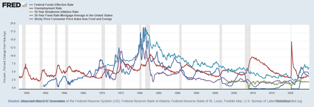
plot represents several key economic indicators over time, including the Federal Funds Effective Rate, Unemployment Rate, 10-Year Breakeven Inflation Rate, 30-Year Fixed Rate Mortgage Average, and Sticky Price Consumer Price Index less Food and Energy. The Federal Funds Effective Rate (blue line) shows significant volatility, particularly during the late 1970s and early 1980s, reflecting aggressive monetary policy to combat inflation. The Unemployment Rate (red line) spikes during recessions, notably around 1980, 1990, 2008, and 2020, indicating economic downturns. The 10-Year Breakeven Inflation Rate (green line) and Sticky Price Consumer Price Index (purple line) remain relatively stable, with gradual increases reflecting long-term inflation expectations. The 30-Year Fixed Rate Mortgage Average (turquoise line) generally trends downward, influenced by overall declining interest rates across decades.

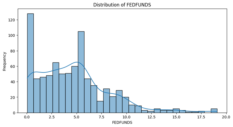
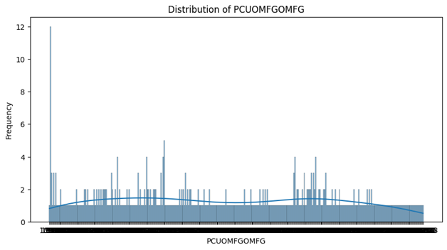
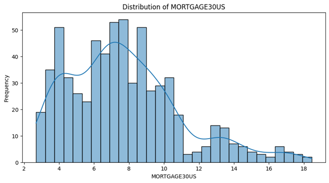
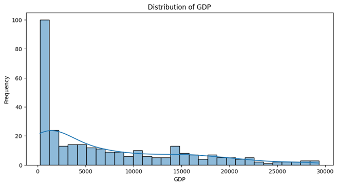
well , these pretty plots indicate the distribution of our data. based on these illustrations we can classify data into the following categories :

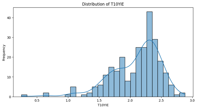
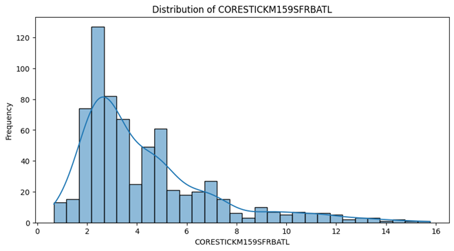
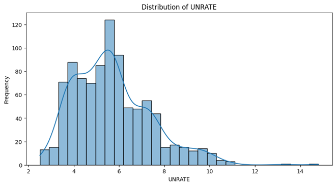
• Unemployment Rate , 10-years-inflation-rate , Sticky Price Consumer Price Index less Food and Energy follow a Unimodal distribution and have one peak and are skewed to either right or left.
• GDP has a very strong peak around zero which means there are a lot of observations which have zero value. This plot is also highly right-skewed that indicates a few data points represent significantly higher GDP values.
• Fed Fund and 30-Year Fixed Rate Mortgage Average in the United States both follow a bimodal distributions with two peaks in the left side and both are skewed to the right.
• Despite of the other data, the distribution plot of Producer Price Index by Industry is totally spread out with no clear peak, suggesting a uniform-like distribution. The data points are spread across a wide range, indicating variability in the index. The plot shows some extreme values but lacks a clear direction of skewness.

Now let’s look deeply into the data and see how these data are related to each other. To do so we use Pearson Correlation Matrix which reveals how different economic factors are related to one another.. (I will explain further what Classified Rate Change and Converted Rate are and how there are calculated , for now just consider Classified Rate Change as our final target.)

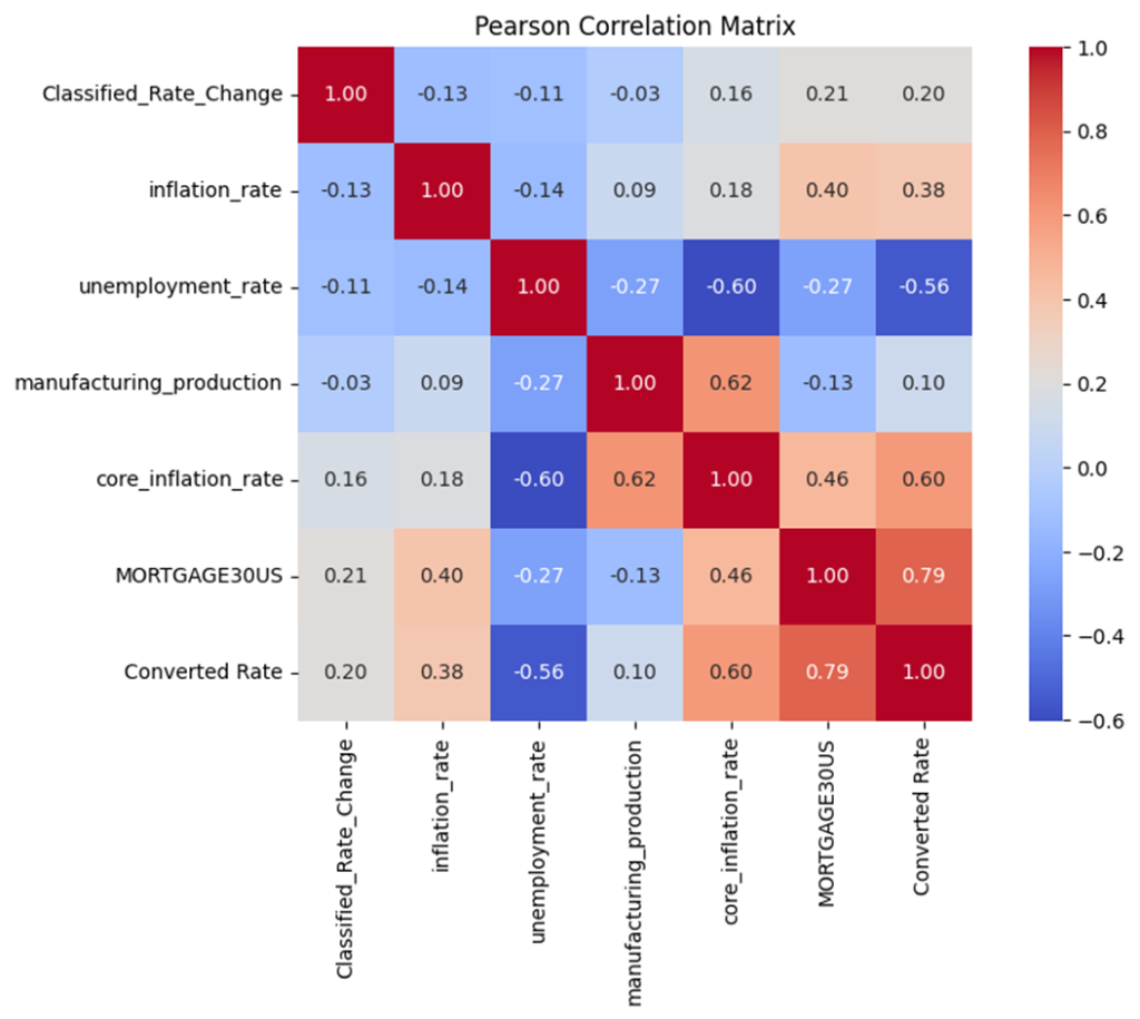
• 30-Year Fixed Rate Mortgage and Converted Rate show a very strong positive correlation (0.79), which makes sense since these are both interest rate measures that tend to move together
• Core inflation rate and manufacturing production have a notable positive relationship (0.62), suggesting that higher manufacturing activity often coincides with higher core inflation
• Unemployment rate and core inflation rate have quite a strong negative correlation (-0.60), indicating that when unemployment goes down, core inflation tends to go up (and vice versa)
• Unemployment rate and Converted Rate also show a strong negative relationship (-0.56), suggesting that higher unemployment often corresponds with lower interest rates
• MORTGAGE30US and core inflation rate show a moderate positive correlation (0.46), which tells us that mortgage rates tend to rise somewhat with core inflation
• Regular inflation rate and 30-Year Fixed Rate Mortgage have a moderate positive correlation (0.40), though interestingly it’s not as strong as the relationship with core inflation
• The Classified_Rate_Change has relatively weak correlations with most other factors, with the strongest being just 0.21 with 30-Year Fixed Rate Mortgage
• Manufacturing production and inflation rate have a very weak correlation (0.09), suggesting these two factors don’t move together as much as one might expect

Classified Rate Change (target classes)

The most crucial analysis in classification tasks is to see whether our classes have equal abundancy or they are imbalanced which leads us through additional steps to deal with this. As you know , imbalanced classes can introduce bias in our model’s decisions, leading to an overemphasis on the majority classes. This bias can result in inaccurate predictions on the test data.

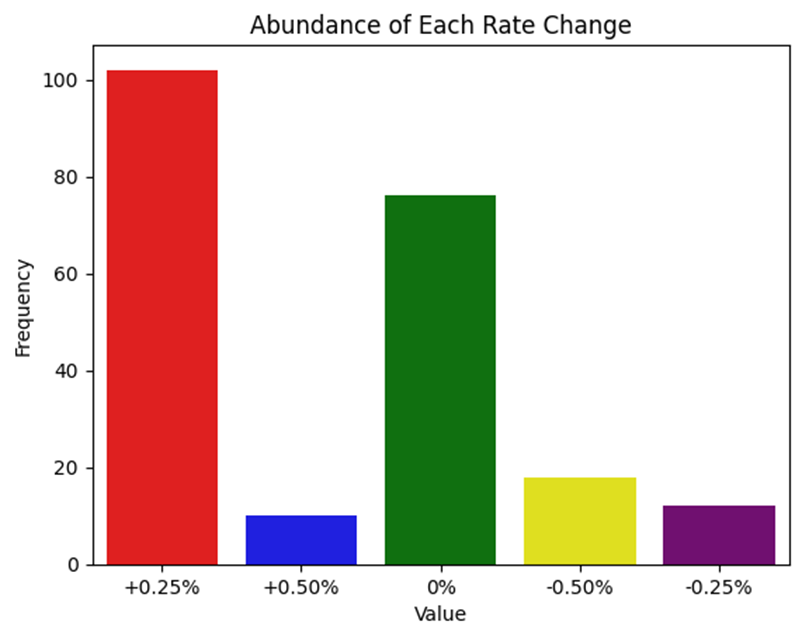
As you can see , this stunning picture indicates that the classes are highly and significantly imbalanced. more than 100 samples are labeled with +0.25 and nearly 80 samples are labeled with 0% changes, while the other classes each has under 20 samples.

Sooo… What can we do ? There are a few ways we can leap into action and tackle this issue :

1. Over-sampling: Over-sampling is like giving a little extra attention to the minority class by randomly duplicating its examples in the training dataset. This helps ensure that the model pays more attention to those less frequent but important cases!
2. Down-sampling: Down-sampling takes a different approach by trimming down the majority class, randomly removing some of its examples to create a more balanced dataset. It’s like saying, “Let’s not overwhelm our model with too many similar stories!” .this method is not recommended for a dataset with low amount of samples. also it contains data loss which should be adopted cautiously.
3. Class- weighting :  involves adjusting the importance of each class during model training by assigning different weights to them. This way, the model learns to treat the minority class with extra care, making it feel just as important as the majority class!

Text Data :

Ok It’s enough with economic data , let’s go forward toward analyzing our text data to see how they are. After tokenization and removing all redundant words, we plotted the most frequent words. The left plot shows the top 20 words which are most frequent and the right plot is the word cloud image of the most frequent tokenized word.

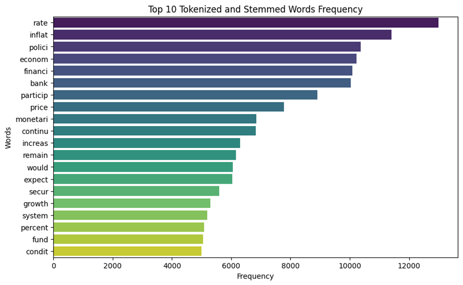
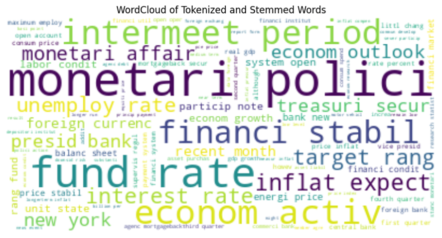
Rate , inflation , policy, monetary, economic , finance , active , stability, fund , target , unemploy , period , intermeet are the most used words in the documents .

Models

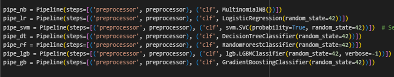
let’s directly jump into the most exciting part which is … yesss models. For classification tasks we have a bunch of good and reliable models that we can use them for our purpose. among all available models, we used these models each for a particular reason:

• Logistic Regression is used for its simplicity and baseline comparison.
• Random Forest provides interpretability and robustness for tabular data.
• XGBoost are advanced gradient boosting methods, often performing well in structured data.
• SVM are great for classification because they effectively find optimal decision boundaries, specially for text classification tasks.
• Decision Tree are user-friendly and intuitive, allowing for easy interpretation of decisions.

To examine the performance of different models all at once we built a pipeline with these models.

We did use three different approach for the modeling part:

1. Using only the text data as feature : in this case we had to shift the target column one level up because we didn’t access the FOMC docs in December and could not consequently predict it. Shifting the target one level up means we used the documents of previous month for the target of current month. in this approach ,we only applied class-weighting method to deal with imbalanced-class.
2. Using only economic and historical interest rate as lags data for the features : In this case, we used time series prediction algorithms, like LSTM, to forecast the features for the upcoming month. Instead of shifting the target, we utilized these predicted feature values to predict the rate change for December. Additionally, we explored three methods for addressing imbalanced classes: down-sampling, over-sampling, and class weighting.
3. A hybrid method of both text and economic  factors: we used the shifting target method for this case too. We only applied class-weighting method to deal with imbalanced-class.

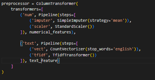
We did run Count Vectorizer and TF-IDF with these models so the output from that was directly fed into each of these models. To optimize these models, we included Standard Scaler.

Results on Text Data

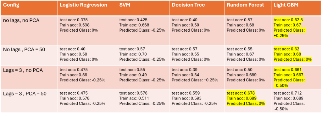
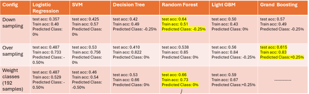
Results on Economic Data

Results on Hybrid Data

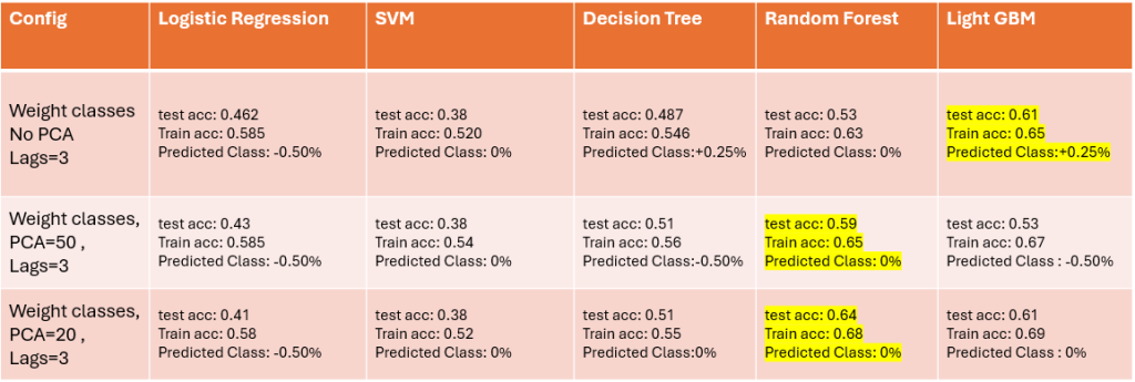
Generally the accuracy on economical data are higher than the two other approach. and it make sense because we didn’t shift the target and used the data of each month to predict the target of that month. Based on the results (which I admit are not good at all) using the economic data with the weight-class approach and using Random-Forest model is the best config, and the predicted class either respect to this config or by majority vote of all configs and all models is 0% which means that the interest rate in December wouldn’t be changed. (however the real interest rate in December decreased by -0.25% – we will point some reasons that leaded to this wrong prediction in Challenges section)

Observations and further Analysis

We used LIME for model interpretability and tested it only on the best config (RF, weight-classes, economic data plus lags) to predict test sample and see which features affect the most. These are the mapping classes :

•     ‘+0.25%’ : 0,
•     ‘+0.50%’: 1,
•     ‘0%’: 2,
•     ‘-0.50%’: 3,
•     ‘-0.25%’: 4

And this is the result of LIME analysis:

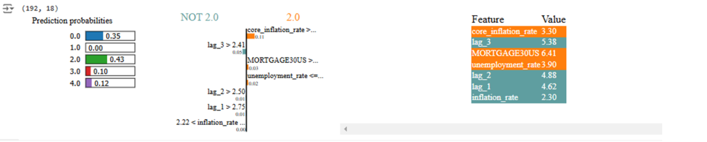
The LIME chart highlights which features most influence the prediction. The core_inflation_rate و lag_3, 30-years mortgage and unemployment rate have the most impact and are significant contributors to the decision, where a higher core inflation rate suggests the prediction towards class 2.0 (0%) , the higher lag_3 values seem to influence the prediction towards not class 2.0, as indicated by the color-coded bars. however 30-years mortgage and unemployment_rate have less impact on result.

Challenges

There were a few challenges which we encountered during the work.

• The most important one was no available feature for the December and we have to predict the economical features and predict the target by predicted features which would lead to less accurate result
• Text data for December couldn’t be predicted nor existed so we had to use shifting target techniques.
• The classes of the prepared dataset were highly imbalanced and dealing with them was challenging
• The size of dataset was not large enough to be able to trust to results confidently
• GDP feature was reported quarterly and we had to apply forward-fill and backward fill approach to convert it to monthly data

Final Note and Conclusion

In this post, we tried to explore the challenges associated with using AI for predicting FOMC interest rate decisions. We discussed the complexities of economic data, the intricacies of machine learning models, and the unpredictability of market reactions. While the article provides a solid foundation, it could benefit from more detailed case studies and real-world examples to enhance understanding. Future work could focus on integrating advanced AI techniques and more diverse datasets to improve prediction accuracy.