The transition to net-zero buildings is a critical step toward achieving global sustainability goals, particularly in the European Union, where the built environment accounts for a significant portion of energy consumption and greenhouse gas emissions. Improving building energy efficiency not only reduces environmental impact but also lowers operational costs and enhances occupant comfort. With advancements in data analytics and machine learning, it is now possible to analyze building energy performance at an unprecedented scale, identify inefficiencies, and propose targeted interventions. This effort is essential for meeting regulatory standards, combating climate change, and driving innovation in sustainable construction practices.
In this work, I worked on Catalunya dataset with 1,336,925 records and 69 features. I applied a comprehensive EDA and feature engineering on it, however, in some cases where I felt there wasn’t enough data for a specific part, I used the Ireland dataset alternatively, which contains 1,264,371 records and 214 features, to address that question. In the last, I trained various ensemble models (RandomForest, CatBoost, XGBoost) on the Catalunya data and used their aggregation to predict the amount of energy consumption (KW/m2) and CO2 emission of each Catalan house.
The outline of this post is as follow:

Brief Dataset Overview
Catalunya dataset contains1,336,925 records and 69 features. Features can be divided into six categories:
- Geographic information: Province, County, Street, latitude and longitude, address, Municipality, …
- Energy consumption/ CO2 emission: these features exist in both categorical rating values and real continues values
- Rating: Non-renewable primary energy rating letter (AG), CO2 emission rating letter (AG), Qualification of CO2 emissions associated with the heating / refrigeration / lightening/ Domestic Hot Water service (AG), Qualification of non-renewable primary energy consumption by the heating / refrigeration / lightening/ Domestic Hot Water service (AG), …
- Real Continuous: Non-renewable primary energy value [kWh / m2 · year], Value of CO2 emissions [kg CO2/m2 any] , Energy at the point of consumption equivalent to energy consumption [kWh / m2 · year] , CO2 emissions associated with the heating / refrigeration / lightening/ Domestic Hot Water service [kg CO2 / m2 · year] , non-renewable primary energy consumption by the heating / refrigeration / lightening/ Domestic Hot Water service [kWh / m2 · year]
- Financial Cost: Approximate annual cost of energy per home
- House Features: It has an electric vehicle charging point (Yes / No), It has solar thermal installation (Yes / no), It has photovoltaic installation (Yes / no), Average window transmittance [W / m2 · K], It has biomass installation (Yes / no), …
- Renovation Measures: Rehabilitation actions, Energy rehabilitation has been carried out [Yes / no]
- Date: year of construction , Date of registration
Missing Values
Most columns of Catalunya dataset have few missing values only a few columns are sparse. Figure 1 illustrates the percentage of missing values of each feature. 6 features have more than 90% missing values, which are listed below. The two most important columns among these are ACTUACIONS_REHABILITACIO (Rehabilitation actions) and ANY_CONSTRUCTO (Year of construction)
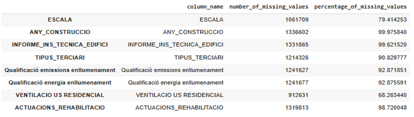
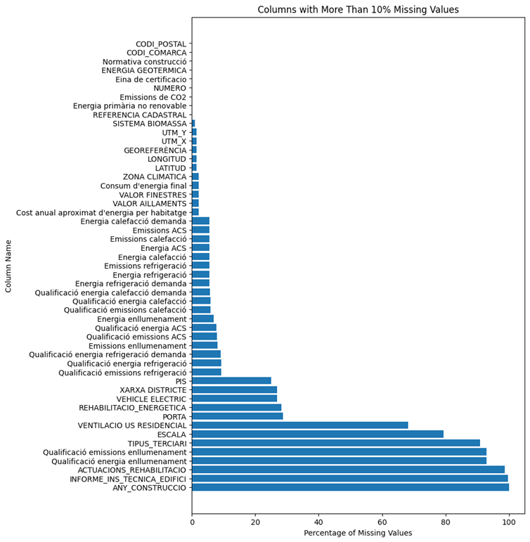
.By looking at Table 1 and Figure 1, We can see that only 8 columns have more than 50% missing values and 56 columns have less than 10% missing values. 5 columns also have between 30% to 50 percent missing values.
Data Types
40 features have string datatype and 29 of them were either float64 or int64. Among these 40 string features, 13 of them were ordinal features (except climate zone , the other 12 features are energy-rating features that their name starts with Qualificació). These features have values from A-G which A demonstrate the best quality and G is the worst quality. All these ordinal features were encoded with label encoding method.
9 of these 40 features were non-ordinal features with low cardinality so I encoded them with one-hot encoding method. These features are:
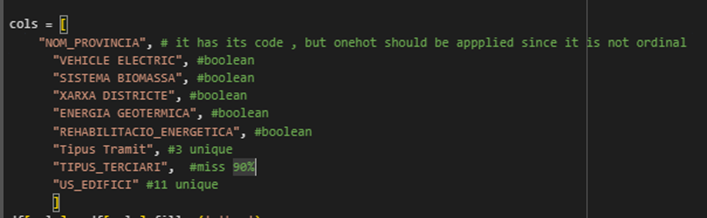
4 of these string features were non-ordinal but with high cardinality These feature later were encoded using frequency encoding techniques. The last two features in Figure 4 had integer datatype but they were categorical data with a huge gap between their values’ frequency. These two also were encoded by frequency encoding.
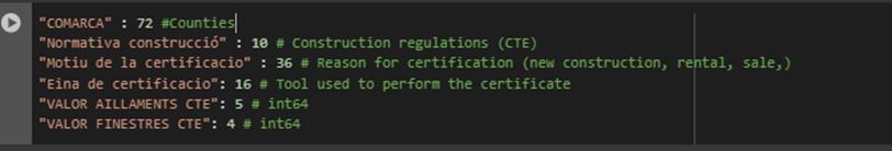
Figure 5 shows the frequency of values of some of these features. Based on the following images, Barcelona being the most represented province, far outnumbering others like Girona, Tarragona, and Lleida. In terms of energy certification tools, “CE3X” is the most commonly used, followed by “CE3” and other tools. The construction regulations also show a clear trend, with pre-1979 regulations being the most frequent, followed by more recent standards such as the NBE-CT-79 and others
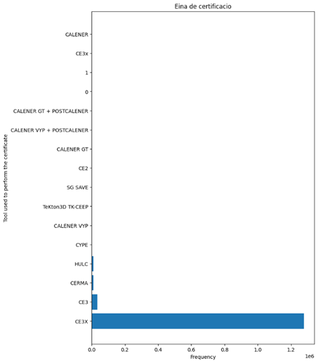
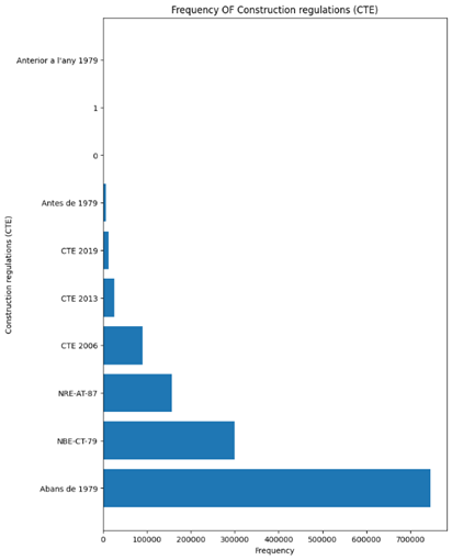
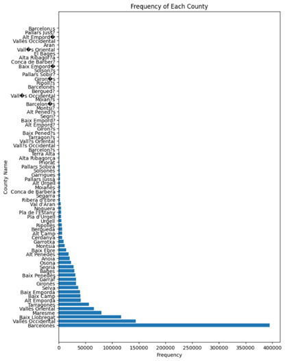
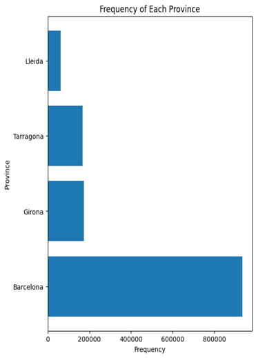
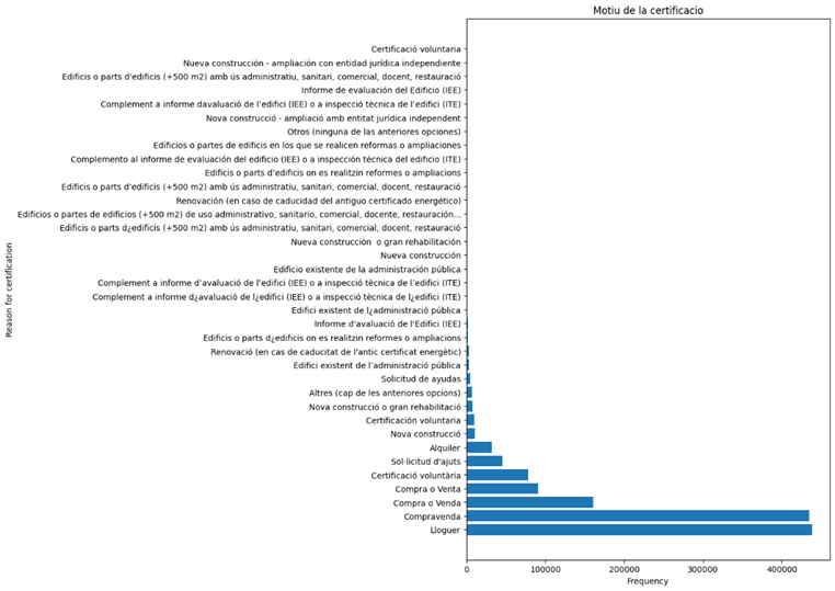
Figure 5 Frequency bar plot of features
EDA
For the first two questions in the EDA part (i.e. 1- Identify the most cost-effective renovation measures in terms of energy reduction (kWh/m² saved per cost unit, 2-Determine the most financially efficient renovation measures in terms of energy cost savings per investment dollar.).), I focused on ACTUACIONS_REHABILITACIO (Rehabilitation actions) feature. This feature as I mentioned before, has 98.7 % missing values, where comparing it with REHABILITACIO_ENERGETICA feature which has boolean data type and implies whether houses have applied renovation actions or not, indicates that these amounts of missing values imply 98.7% of houses in Catalunya haven’t applied renovation actions.

ACTUACIONS_REHABILITACIO Feature
17,112 records in this feature have values that means this amount of houses have already done renovations. This feature has unstructured messy text data in Catalan language, some records have multiple renovations separated with || which need to be split and organized. Here is a raw record of ACTUACIONS_REHABILITACIO.
Aïllament en façanes i/o coberta. || Renovació de finestres i/o proteccions solars. || Millora de les instal·lacions (calefacció, climatització, ACS, enllumenat,…)
The following preprocessing steps were applied on this feature:
- Removing redundant characters like [], {} , || , …
- Translation of all Catalan text into English text using googletrans library in python
- Splitting the records with multiple renovations into multiple records.
- Grouping and aggregating records with similar context but different wording/structure (there were numerous records of Photovoltaic Installation which had different wording, I tried to group them as much as possible but some records with very different shape still remained)
- Counting each group’s frequency and pick the top most frequent groups: since after grouping them there were still plenty of categories of renovation (about 1114 unique categories) which most of them was very infrequent and rare, I set a small threshold (0.0005) and only picked those which had a frequency of at least 0.05% of the total dataset. I grouped the rest of them in ‘other’ category. 11 renovation categories were chosen for further analysis
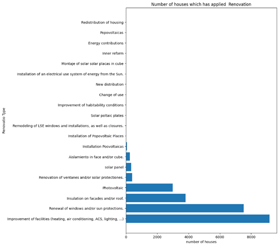
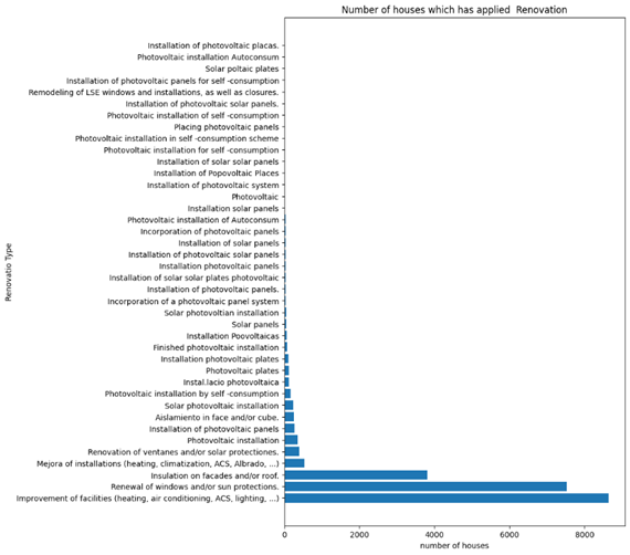
Figure 6 Frequency plot of renovation measures. The right figure is before grouping, the left figure is after grouping
3-1 Identify the most cost-effective renovation measures in terms of energy reduction (kWh/m² saved per cost unit).
There were multiple features in the dataset that demonstrate energy consumption and CO2 emissions. Each of these was investigated separately based on the processed categorized renovation measures to see which measure is more effective.
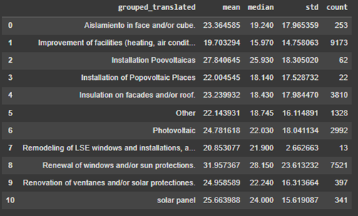
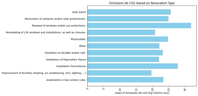
Figure 7, demonstrates the amount of CO2 emission based on each type of renovation. The upper table shows mean, median, std of CO2 emissions [kg CO2/m2 any] and the number of houses that have applied that type or renovation. The lower figure visualizes the mean of CO2 emission of houses placing into that group of renovation. Looking at these two figures, Improvement of facilities (heating, air condition, …) has worked better than the other renovations in both terms of mean and median to reduce the emission of CO2. This measure is the most popular one among Catalan houses where more than 9000 houses have applied it.
based on each renovation measure
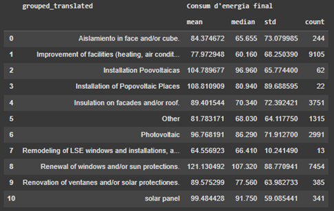
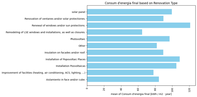
Figure 8 illustrates the Energy at the point of consumption equivalent to energy consumption (Consum d’energia final) associated with each type of renovation. The upper table provides the mean, median, standard deviation of energy consumption in a year (KW/m2-year), and the number of houses that have undergone that specific type of renovation. The lower figure visualizes the mean energy consumption of houses categorized by renovation type. Observing these two figures, it is evident that the Remodeling of LSE windows and installations as well as closure, has been more effective than other renovations in term of mean. However, this renovation is the least frequent with only 13 houses having applied it. Setting it aside, Improvement of facilities (heating, air condition, ACS, lightening) outperforms the other measures in terms of both mean and median.
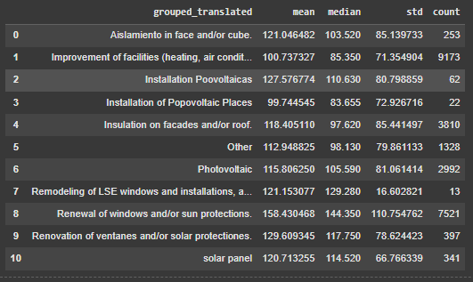
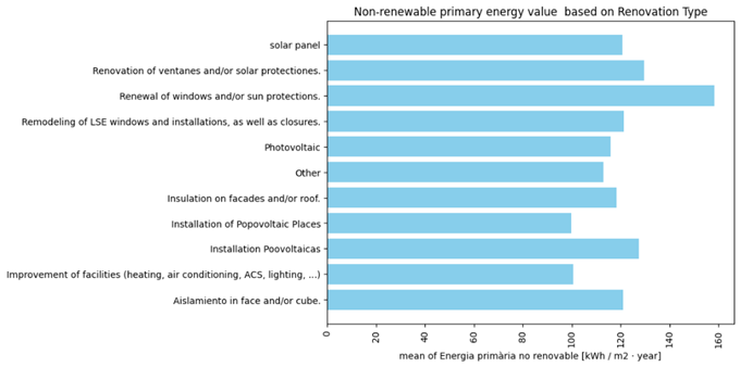
Figure 9 shows the Non-renewable primary energy (Energia primària no renovable) consumption in a year (KW/m2-year), associated with each type of renovation. Based on these images, Installation of Popovoltaic Places with mean 99.7 KW/m2 and median 83.6 KW/m2 in a year and Improvement of facilities (heating, air condition, ACS, lightening) with mean 100.7 KW/m2 and median 85.3 KW/m2 in a year have major roles in reducing Non-renewable primary energy consumption.
By comparing Figures 7-10, one can conclude that Improvement of facilities (heating, air condition, ACS, lightening) can be considered as the best actions and Renewal of windows and/or sun protections is the least effective measure in reducing energy consumption and CO2 emissions. These measures have been applied in nearly 9000 and 7500 houses respectively.
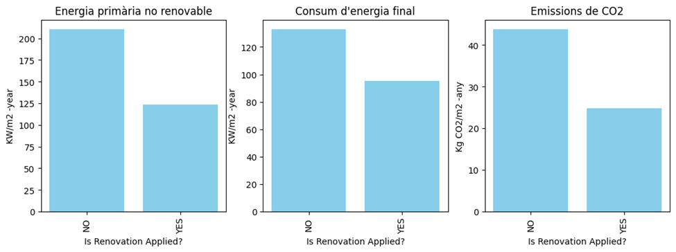
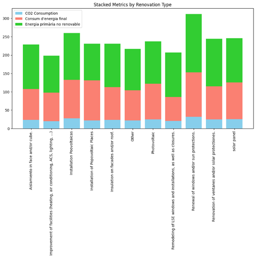
Figure 11 presents a comparison of three key metrics—non-renewable primary energy, final energy consumption, and CO2 emissions—with or without renovation actions. The bars show a clear reduction in all three categories when renovation is applied. Specifically, non-renewable primary energy consumption drops from over 200 units to below 125 units, final energy consumption decreases from around 130 units to just below 100 units, and CO2 emissions are reduced from over 40 units to around 30 units. This indicates that renovation actions lead to significant improvements in energy efficiency and a reduction in environmental impact.
3-2 Determine the most financially efficient renovation measures in terms of energy cost savings per investment dollar.
Feature ‘Cost anual aproximat d’energia per habitatge‘ indicates Approximate annual cost of energy per home. In order to determine the most financially efficient renovation measures, I calculated the mean, median and standard deviation of each renovation measure in term of this feature.
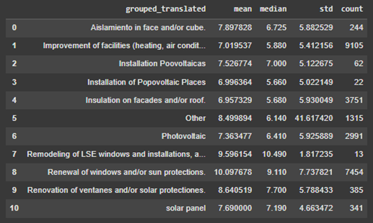
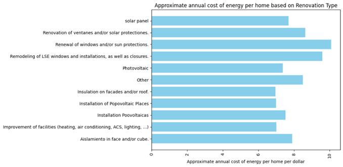
Figure 12 illustrates the impact of different renovation actions on annual cost of energy per home. It is evident that Window-focused renovations, such as “Renewal of windows and/or sun protections” and “Remodeling of LSE windows,” show substantial energy effects but are among the most expensive options, with costs around 10-11 dollars per home. In contrast, solar panels are more cost-effective at approximately 8 dollars per home, while insulation on facades/roofs offers moderate costs of about 7 dollars. The “Improvement of facilities” is the most prevalent renovation type in Catalunya, applied to a large number of homes. Not only is it effective in reducing energy consumption, but it is also relatively cost-effective, with costs averaging around 7 dollars per home. This combination of efficiency and affordability likely explains why it is the preferred choice for many homeowners in the region.
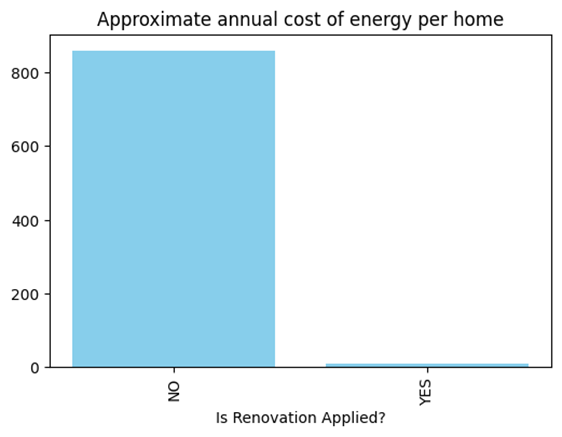
Figure 13 dramatically illustrates the financial impact of renovations, showing approximate annual energy costs per home with and without renovation. Homes without renovations (“NO”) have costs around 850 units (likely dollars or euros), while renovated homes (“YES”) show drastically reduced costs near zero. This stark contrast demonstrates that renovations, despite their varying effectiveness shown in Figure 12, collectively result in substantial energy cost savings. The magnitude of this difference suggests that virtually any of the renovation categories from the first image would likely produce significant financial benefits for homeowners, though some (particularly window-related renovations) may offer superior performance.
3-3 Analyze which building elements have the greatest impact on energy consumption.
For this part, Catalunya dataset lacked the features that address building elements. It contained only four boolean features which doesn’t completely reflect building elements, e.g.
- VEHICLE ELECTRIC: It has an electric vehicle charging point (Yes / No)?
- SISTEMA BIOMASSA: It has biomass installation (Yes / no)?
- XARXA DISTRICTE: It has connection to a district network of generation of heat and / or cold (Yes / no)?
- ENERGIA GEOTERMICA : It has geothermal installation (Yes / no)?
Therefore, I also used the Ireland dataset since this dataset has more features related with building elements. Figures 15-19 represents the information of the Ireland dataset.
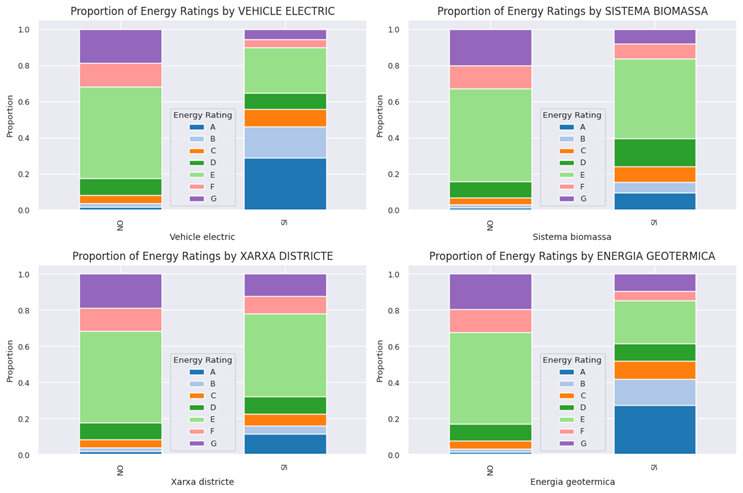
Figure 14 presents a comparative analysis of energy ratings across four distinct elements under two different conditions, denoted as “NO” and “SI.” A visual inspection reveals that the distribution of energy ratings varies significantly among the elements and between the two conditions. In general, a shift towards higher energy ratings (e.g., A and B) is observed in the “SI” condition compared to the “NO” condition across all elements, suggesting an improvement in energy performance.
Specifically, the element labeled “Energia Geotermica” exhibits the most pronounced shift, with a majority of instances moving to the highest energy rating under the “SI” condition. Similarly, “Vehicle Electric” also demonstrates a substantial improvement, with a large proportion achieving high energy ratings in the “SI” scenario. The remaining two elements, “Xarxa Districte” and “Sistema Biomassa,” also show positive trends, albeit to a lesser extent, with a noticeable migration towards better energy ratings when comparing the “NO” and “SI” states.
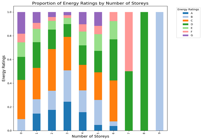
Figure 15 illustrates the proportion of energy ratings relative to the number of storeys in a building. Buildings with zero storeys have a wide range of energy ratings, while buildings with one or two storeys are more likely to have B or C ratings. As the number of storeys increases, the proportion of lower energy ratings (E, F, G) tends to increase, with a noticeable shift towards lower ratings for buildings with 6 or more storeys. Buildings with nine stories are rated B, which probably could be commercial building with high renewable energy technologies, or simply be an outlier.
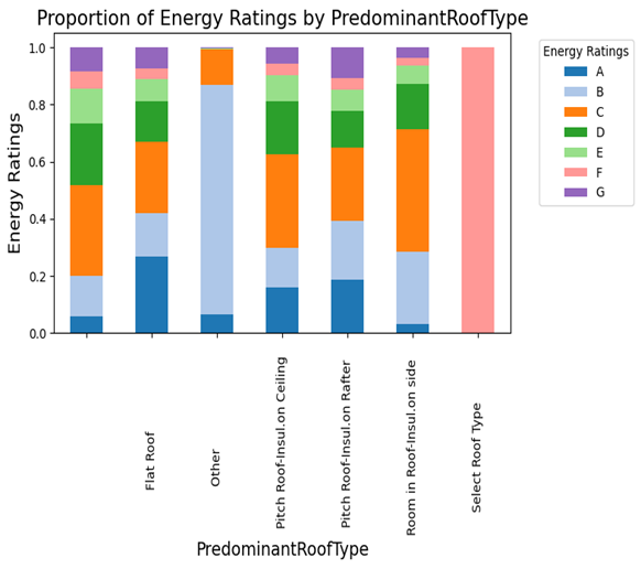
Figure 16 presents the proportion of energy ratings based on the predominant roof type. Flat roofs and “other” roof types show a diverse mix of energy ratings, while pitch roofs with insulation on the ceiling or rafter tend to have better energy ratings (A, B, C). Buildings with “room in roof insulation on side” also show a mix of ratings. The “select roof type” category is overwhelmingly dominated by the E rating, indicating this roof type is associated with poorer energy performance compared to the others.
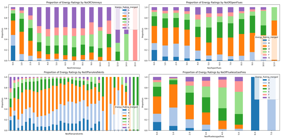
Figure 17 presents a series of stacked bar charts illustrating the relationship between different building elements (number of chimneys, open flues, fans and vents, and flueless gas fires) and the energy ratings of buildings. Based on this image:
- Number of Chimneys: The plot illustrates that buildings with very few or a high number of chimneys tend to have lower energy ratings (more F and G ratings). Buildings with a moderate number of chimneys (around 4-8) appear to have a slightly better distribution of energy ratings.
- Number of Open Flues: The plot shows a general trend where buildings with fewer open flues tend to have better energy ratings (more A and B ratings). As the number of open flues increases, the proportion of lower energy ratings (E, F, and G) also tends to increase.
- Number of Fans and Vents: This plot indicates that buildings with very few fans and vents tend to have higher energy ratings. As the number of fans and vents increases, the energy ratings become more distributed, with a larger proportion of lower ratings.
- Number of Flueless Gas Fires: The plot suggests that buildings with no flueless gas fires have the best energy ratings. As the number of flueless gas fires increases, the proportion of lower energy ratings increases significantly.
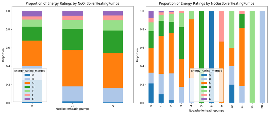
Figure 18 presents two stacked bar charts comparing the distribution of energy ratings in buildings based on the number of “Oil Boiler Heating Pumps”(left) and “Gas Boiler Heating Pumps”(right). Left chart indicates that houses have (0, 1, or 2) Oil Boiler Heating Pumps. With zero pumps, the majority of buildings have a C rating, followed by D. As the number of these pumps increases to 1 and then 2, there’s a slight shift: the proportion of B-rated buildings increases noticeably, while the proportion of C-rated buildings decreases a bit, suggesting a potential correlation between having these pumps and achieving a slightly better energy rating.
The right chart shows the distribution of energy ratings based on the number of ” Gas Boiler Heating Pumps.” Here, we see more variance. Buildings with very few or many of these pumps (0, 1, 11, 14, and 20) tend to have a higher proportion of A and B ratings. In contrast, buildings with an intermediate number of these pumps (around 6 to 10) appear to have a larger proportion of lower energy ratings like C and D. This suggests a more complex relationship where having a certain number of ” Gas Boiler Heating Pumps ” might not linearly correlate with better energy performance; other factors are likely at play.
Feature Engineering
Categorical Data
there were around 28 categorical features in this dataset (both string and float/ int type). 13 of them were ordinal which indicates rating of energy consumption/ CO2 emissions and all these features encoded by label encoding to preserve the order, nan values in these features replaced with a very big number i.e. “99999”. 9 of features were encoded by one hot encoding since they were how cardinal and non-ordinal features, nan values in these features were removed after applying one-hot encoder. 6 features with high cardinality were encoded using frequency encoding where the frequency of each record replaced with the real value.
after performing the encoding process, I standardized these features using standard scalar.
Continuous Data
Most of the continuous features in the data show a large concentration of data around the lower values (close to zero) and a long tail extending towards higher values. Where the data is highly skewed. Here are the histogram plot of some raw features before any transformation:
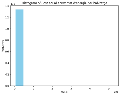
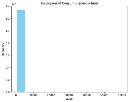
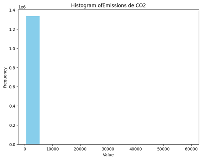
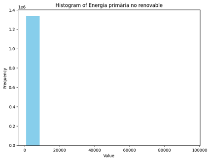
Figure 20 the distribution of raw continuous data
Other features had the same distribution which make it hard to interpret and train a model on them. To deal with this issue, I passed each feature through 4 processing steps to remove the negative values, avoid the outliers, uniform the distribution and standardize the scale of them. Here is the code snippet for doing so:
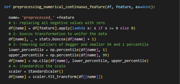
After applying these steps features became more normalized and ready to be trained. Figure 21 shows some of these features after transformation.
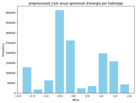
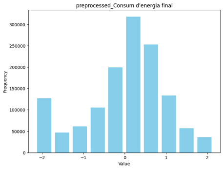
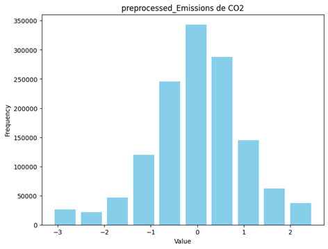
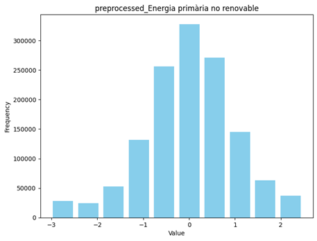
Figure 21 the distribution of preprocessed continuous data
The feature of cost still doesn’t follow a uniform distribution but I didn’t transform it again to preserve the nature of the data.
New Features
By looking at the data some new potential features were created which some of them turned out to have significant impact on the modeling process. Here are the list of features:
- Age: this feature was created by subtracting the current year (2025) from the year of DATA_ENTRADA (Date of registration).
- Energy Efficiency: for each of the four metrics of heating(calefacció), lightening (enllumenament) , domestic hot water (ACS) and cooling (refrigeració) I created new feature to address the efficiency of these metrics by dividing their energy consumption to their CO2 emissions. For example here is how heating-efficiency feature was made: df[‘heating_efficiency’] = df[‘Energia calefacció’] / df[‘Emissions calefacció’]
- Total Energy : this feature was created by adding up the four above energy consumption’s metrics. i.e. heating(calefacció), lightening (enllumenament) , domestic hot water (ACS) and cooling (refrigeració)
- Total Emission : this feature was created by adding up the four above CO2 emissions’ metrics.
These features then transformed and normalized to be prepared for the model.
Models and Analysis
For modeling section, I used three ensemble model XGboost, Catboost, Random Forest and one stacking model which aggregates these three trained models using a simple linear regression for more robustness. The reason of choosing these three ensembles is due to their robust performance, efficiency, and ability to handle complex data. XGboost and Catboost also execute too fast which make them appropriate for big scale of data.
The target that should be predicted is final Energy Consumption (Consum d’energia final). I’ll explain the modelling steps of predicting the target in follow.
Consum d’energia final
Feature Selection
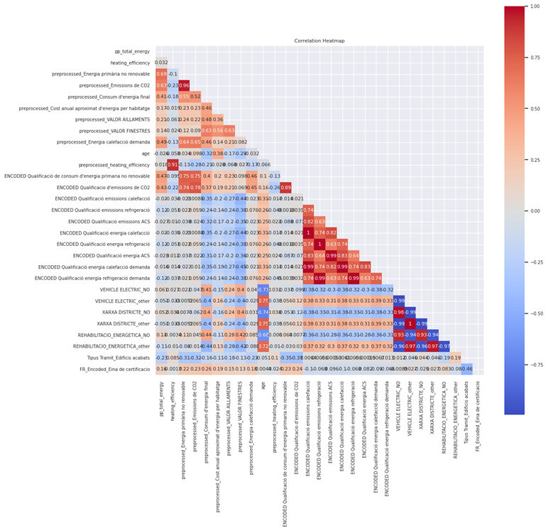
First of all, I extracted the most correlated features with Consum d’energia final. Figure 22 illustrates the correlation bar chart of this feature. As it can be seen, there are lots of features that are moderately to highly correlated with the target including age, heating efficiency, Cost, total energy, total emission and … . I applied a filter of 0.15 of correlation to choose a smaller subset of features to work with. The filtering process gave me a list of 32 features (including the target itself). In the next step, I calculated the selected features pairwise correlation using the heatmap to remove high-correlated features. Figure 23 shows the result of pairwise correlation matrix. As the heatmap plot shows, there are multiple features which are highly correlated to each other and must be removed.
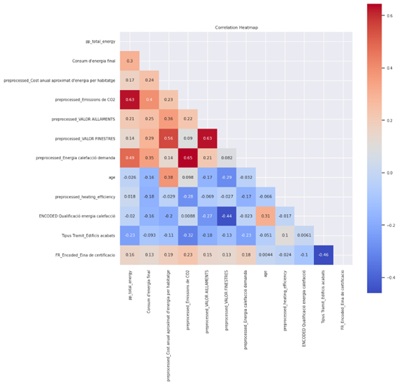
After removing the highly-correlated features, we ended up with this correlation matrix which determines everything is ready for training a model. The red points show a correlation of 0.63-0.65 but I decided to ignore them and run the model to see the result.
Model Configuration
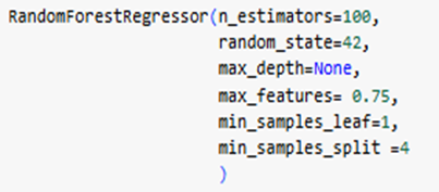
I applied a grid search for each of the ensemble models to find the best hyper parameters. Since the dataset was relatively large, grid searching took too much time especially for RF model. To cope with this issue, I used a small subset of dataset around 213,908 records to find the optimal hyper-parameters and then applied them to the model while training on real data. I split 0.2 of data as the test set with the size of 267,385 records and the rest of data as the train set. Three accuracy metric MSE, MAE and R2 represents the performance of each model. Figure 23 shows the list of tuned parameters for these three models:
Results
Random Forest: this mode performed relatively good on the data, but it took longer time to be executed.
- Mean Squared Error: 0.5702114530173301
- Mean Absolute Error: 0.04407511957616473
- R² Score: 0.21741453975808245
These performances, reveals some inconsistencies. The Mean Squared Error (MSE) is significantly higher at approximately 0.57, indicating larger squared errors and potentially more variance in the predictions. However, the Mean Absolute Error (MAE) is surprisingly low at about 0.044, suggesting that while the model may not be capturing the full range of variability, it is making fewer extreme errors. The R² Score of 0.217 indicates that only about 22% of the variance in the dependent variable is explained by the model, which is a relatively poor fit.
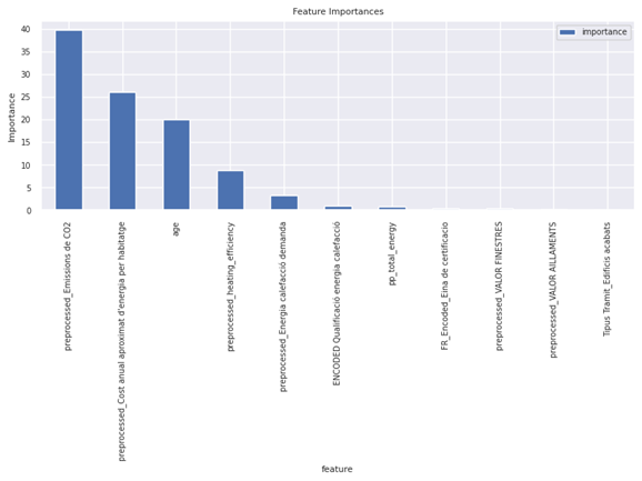
Figure 24 shows important features recognized by RF model. CO2 emission, annual cost and age are the top 3 important features for training.
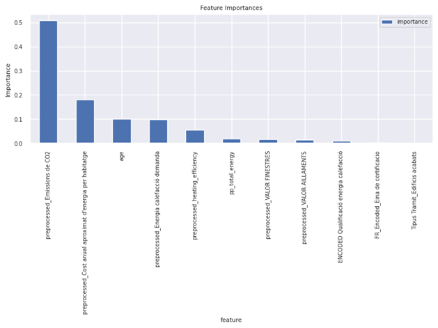
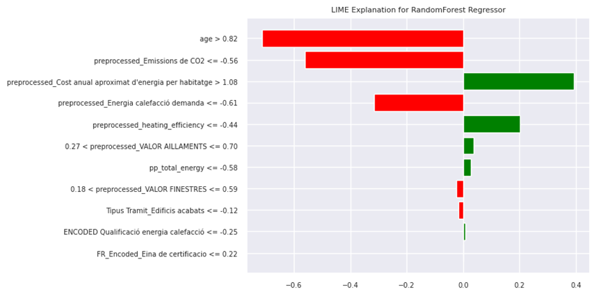
Figure 25 illustrate the interpretability of RF model using Lime for predicting the test sample with index 478,659. The LIME plot indicates the local feature importance for a single prediction. The most significant factors pushing the prediction towards a lower value (shown in red) are ‘age > 0.82’, ‘preprocessed_Emissions de CO2 <= -0.56′, ‘preprocessed_Energia calefacció demanda <= -0.61′, while ‘preprocessed_Cost anual aproximat d’energia per habitatge > 1.08′ contributes the most to increasing the predicted value (shown in green). Other features have smaller positive or negative influences on the prediction.
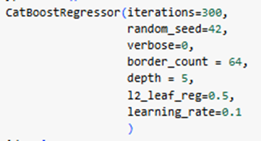
Catboost: this mode performed much better than RF and also much faster. Here are the accuracy results of Catboost:
- Mean Squared Error: 0.083907367536856
- Mean Absolute Error: 0.11042580215548493
- R² Score: 0.7984444379565124
This performance indicates a strong predictive capability of this model. The Mean Squared Error (MSE) of approximately 0.084 and the Mean Absolute Error (MAE) of about 0.110 suggest that the model is generally accurate, with a slight bias towards underestimation given the MAE is slightly higher than the square root of MSE. However, the R² Score of 0.798 indicates that nearly 80% of the variance in the dependent variable is explained by the model, which is a strong indicator of its effectiveness. Overall, these metrics suggest that the Catboost Regressor is well-suited for this regression task, providing reliable predictions with minimal error.
The feature importance list from CatBoost highlights that the same as RF model, Emissions de CO2 and CostandAge are the most influential features, contributing nearly 86% of the model’s predictive power. heating_efficiency also plays a significant role, contributing about 9%. The remaining features have much less impact. This suggests that environmental and cost-related factors, along with age, are key predictors in the model.
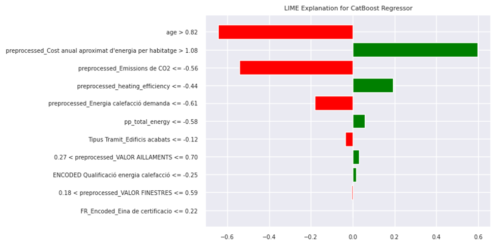
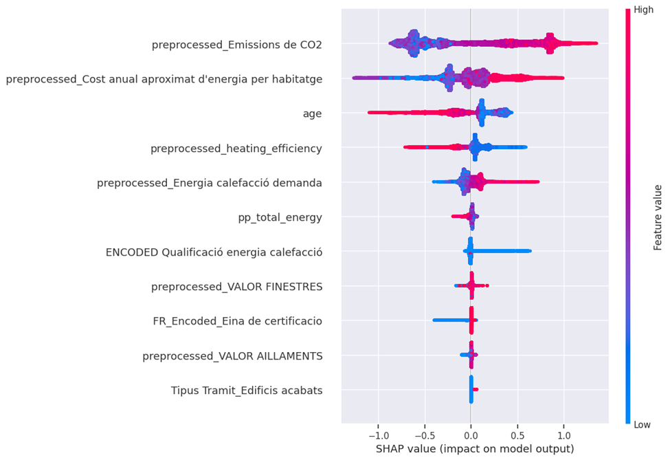
Figure 27 illustrate lime plot of performance of catboost pretrained model. LIME provides a snapshot of feature importance for a specific instance, in this case index of 478,659. Based on the figure, the most important feature contributing positively to the prediction is “preprocessed_Cost anual aproximat d’energia per habitatge > 1.08 and heating efficiency <-0.44 “. The most important features contributing negatively are “age > 0.82″ and “emsission_de CO2 < – 0.56″ .
The SHAP summary plot provides a global view of feature importance and their impact on the model output. Features are ranked by importance. For example, “preprocessed_Emissions de CO2” appears to be the most important feature. The color indicates the feature value (red = high, blue = low), and the x-axis shows the SHAP value (impact on model output). We can see, for instance, that a high value of “preprocessed_Emissions de CO2” tends to decrease the model output, while a high value of “preprocessed_Cost anual aproximat d’energia per habitatge” tends to increase the model output. SHAP values provide a more comprehensive understanding of feature effects across the entire dataset.
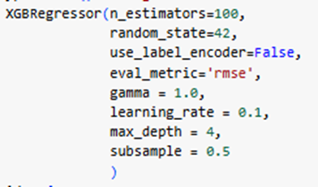
XGBoost: Here are the accuracy results of xgboost model.
- Mean Squared Error: 0.0734779691576633
- Mean Absolute Error: 0.12646084136350222
- R² Score: 0.8182046902330615
The XGBoost model regressor shows strong performance with a Mean Squared Error (MSE) of 0.0735 and a Mean Absolute Error (MAE) of 0.1265. The R² Score of 0.8182 indicates that the model explains about 82% of the variance in the target variable, suggesting a good fit. Compared to the Random Forest (RF) model, XGBoost performs significantly better in terms of MSE and R² Score, although RF has a slightly lower MAE. However, the overall performance of XGBoost is superior due to its higher R² Score and lower MSE.
In comparison with CatBoost, XGBoost has a slightly lower MSE and a higher R² Score, indicating a marginally better performance. CatBoost’s MAE is slightly lower than XGBoost’s, but the difference is not substantial. Overall, XGBoost appears to be the most accurate model among the three, offering a good balance between error metrics and explanatory power. Its ability to explain a larger portion of the variance in the data makes it a preferable choice for this particular regression task.
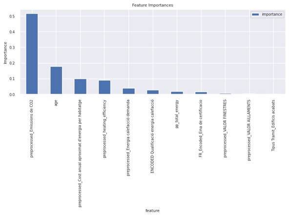
Figure 29 illustrates important features recognized by XGBoost. The feature importance from XGBoost highlights that , Emissions de CO2 and Ageare the most significant influential features, contributing nearly 69% of the model’s predictive power. The remaining features have much less impact. This suggests that the capability of this model highly depends on these two features.
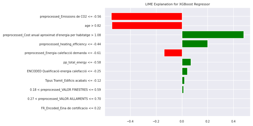
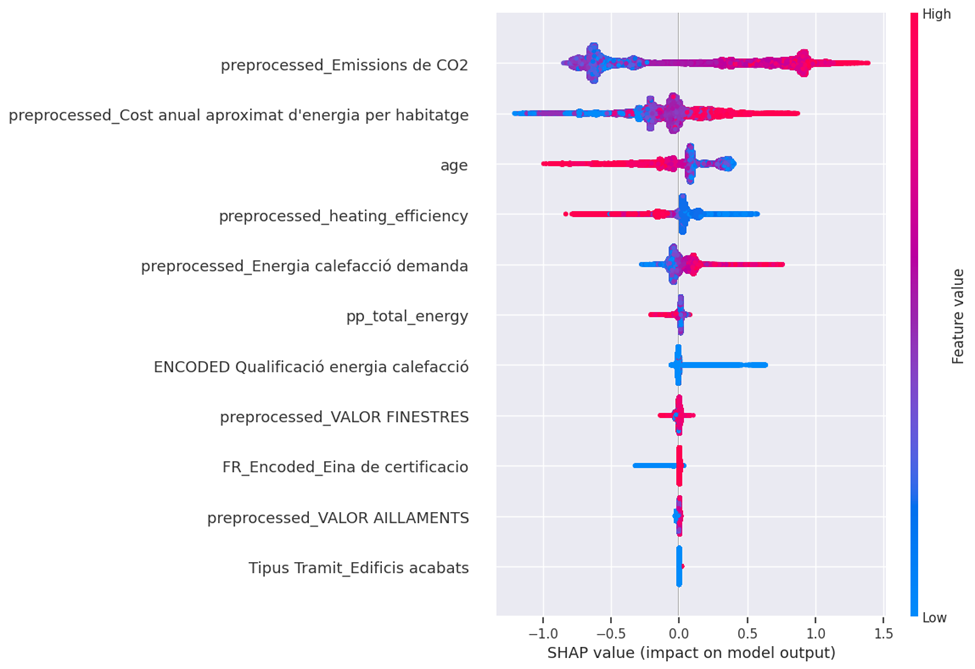
Figure 30 and 31 provide SHAP and Lime interpretation for XGboost model. The SHAP summary plot ranks features by importance and shows the distribution of their impact on the model output. “preprocessed_Emissions de CO2” appears to be the most important feature. Higher values of this feature (indicated by red) tend to decrease the model output (negative SHAP values), while lower values (blue) increase it. Other important features include “preprocessed_Cost anual aproximat d’energia per habitatge” and “age,” both showing a similar pattern where higher values tend to decrease the model output and vice versa. The spread of points for each feature indicates the variability of their impact across different samples.
The LIME plot provides a local explanation for individual predictions. The features are ranked by their contribution to a specific prediction. In this particular instance, higher values of “preprocessed_Cost anual aproximat d’energia per habitatge” contribute positively (green) to the prediction, while higher values of “age” and “preprocessed_Emissions de CO2” contribute negatively (red). The numbers indicate the feature values and their corresponding impact on the model output for a particular instance. For example, when “preprocessed_Emissions de CO2” is less than or equal to -0.56, it negatively affects the predicted value.
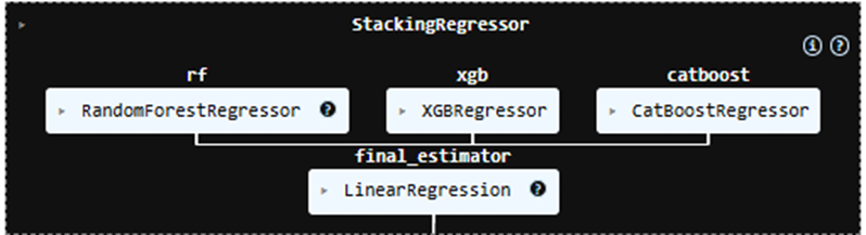
Stacking Regressor Model for Aggregation
After training all three ensemble models, I passed them through a simple linear regression model to have a majority vote of their results. Stacking the models also improve the robustness of models and is a good way to boost the performance. Figure 30 shows a plain structure of the stacking model.
Here is the accuracy of the final estimator on the same set of train and test:
- Mean Squared Error: 0.04083343863681367
- Mean Absolute Error: 0.06565375904333184
- R² Score: 0.8976289933862698
Looking at the results, we can see that the Stacking Regressor demonstrates impressive performance. It achieves a Mean Squared Error (MSE) of 0.0408 and a Mean Absolute Error (MAE) of 0.0657, both of which are significantly lower than those of the individual models. The R² Score of 0.8976 indicates that the Stacking Regressor explains nearly 90% of the variance in the target variable, showing a substantial improvement over the individual models.
Compared to XGBoost, CatBoost, and Random Forest, the Stacking Regressor outperforms all three in terms of MSE, MAE, and R² Score. Specifically, it reduces the MSE by about 45% compared to XGBoost and improves the R² Score by about 8%. This suggests that combining the strengths of multiple models through stacking can lead to more accurate predictions than relying on any single model alone. The Stacking Regressor’s ability to leverage the diverse predictions of XGBoost, CatBoost, and Random Forest results in a more robust and accurate regression model.
you can find the full source code in the Github repository here
Key Findings
- Dataset Characteristics: The Catalunya dataset contained 1,336,925 records and 69 features, including geographic information, energy consumption metrics, financial costs, house features, renovation measures, and construction dates.
- Renovation Measures: “Improvement of facilities” (e.g., heating, air conditioning) was the most effective renovation measure in reducing CO2 emissions and energy consumption while being cost-effective.
- Financial Efficiency: Solar panels and insulation on facades/roofs were identified as financially efficient renovation measures with moderate costs per home.
- Energy Cost Reduction: Renovated homes showed drastically reduced annual energy costs compared to non-renovated homes, with costs near zero for renovated properties.
- Impact of Building Elements: Geothermal installations had the most significant positive impact on energy ratings among building elements analyzed.
- Geographic Trends: Barcelona was the most represented province in the dataset, showing a strong geographical concentration in data distribution.
- Data Encoding Techniques: Label encoding was used for ordinal features while one-hot encoding and frequency encoding were applied to non-ordinal features with varying cardinality.
Conclusion
The study on energy efficiency and emissions reduction in Catalunya highlights the transformative impact of targeted renovation measures and advanced modeling techniques in achieving sustainability goals. By leveraging extensive datasets and ensemble machine learning models, the research provides actionable insights into reducing energy consumption and CO2 emissions. Among the renovation measures analyzed, “Improvement of facilities” emerged as the most effective and widely adopted intervention, significantly lowering non-renewable energy consumption, final energy usage, and annual energy costs. The findings underscore the importance of strategic renovations in enhancing environmental performance while maintaining financial feasibility for homeowners. Furthermore, the integration of data analytics tools like SHAP and LIME enhances interpretability, enabling policymakers to make informed decisions tailored to regional needs.
In addition to renovation measures, the study explored the role of building elements and geographic factors in energy efficiency. It demonstrated that features such as geothermal installations and electric vehicle charging points contribute substantially to improved energy ratings. The comparative analysis with Ireland’s dataset further enriched the findings, offering a broader perspective on building elements’ impact on energy performance. Overall, this research not only provides a roadmap for sustainable construction practices in Catalunya but also serves as a model for other regions aiming to transition toward net-zero buildings.