This was another amazing Ocean Data challenge which was held by Desight team and hosted by Ocean Protocol. this challenge was the 2nd sequel of Formula 1 challenge (In the first sequel , we did a comprehensive EDA on the data, visit these two blog posts : F1 dataset overview , F1 EDA and relationships). In this challenge, we were asked to build machine learning models that predict key elements of pit stop strategies for any driver in the 2024 Mexican Grand Prix (In the time of this challenge, Mexican GP race hadn’t been held yet ). Using the provided datasets, including historical data from previous Mexican Grand Prix races and updated data from the 2024 season, we had to build models capable of predicting the following factors, based on a driver’s starting grid position:
Average Lap Time per Stint: The precision of predicted average lap times compared to actual data.
Number of Stints: How accurately the model predicts the number of stints for a given driver.
Tire Compound Prediction: How accurately the tire compounds are predicted for each stint.
Laps per Stint: The accuracy in predicting the number of laps within each stint.
So before going any further, lets review the outline of this article:
So can we move on ?

Quick Dataset Overview
2024 Races Data
2024 Races dataset contains the information of 15 events which have already been held.
- We used car_data, laps, results and weather dataset since these are the most relevant and influencing on what happens during the race.
- 21 drivers participated in these events
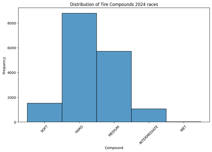
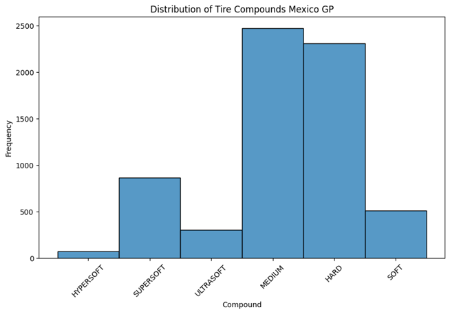
- 5 compounds including [‘SOFT‘, ‘HARD‘, ‘MEDIUM‘, ‘INTERMEDIATE‘, ‘WET‘] have been used for covering the tires.
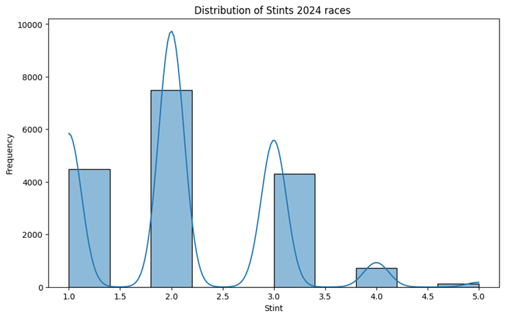
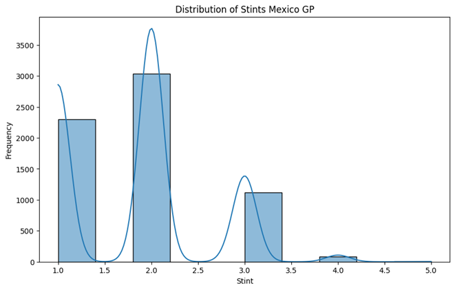
- Maximum number of Stints were 5
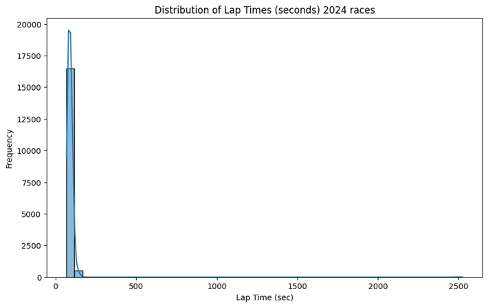
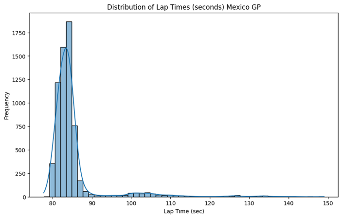
- maximum number of laps were 78
Mexico City Races Historical Data
Mexico City Races dataset contains the information of 5 years races including [2018, 2019, 2021, 2022, 2023]. We used car_data, laps, results and weather dataset since these are the most relevant and influencing on what happens during the race.
- In total 33 drivers have attended in these events
- they have used 6 various compounds including [‘HYPERSOFT‘, ‘SUPERSOFT‘, ‘ULTRASOFT‘, ‘MEDIUM‘, ‘HARD‘, ‘SOFT’ ] in the races.
- Maximum number of Stints during all races were 5
- Maximum number of laps were 71
Merge the datasets
We merged both Mexico City historical data and 2024 races data together to obtain a bigger dataset which benefits from Mexico City environmental Statistics (weather) and all 2024 races statistics that could affects on Mexico 2024 competition’s result. aggregating these two datasets involved multiple steps:
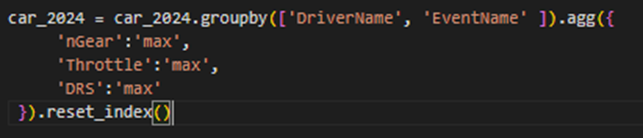
- Since the car-data in both 2024 races and Mexico city races were huge with more than 6 million and 2 million records, merging the raw car-data caused the memory limit error. So we first reduced the size of them by applying a group-by method on [year and driver] for Mexico GP and [event , driver] for 2024 races . We only picked nGear , Throtthle and DRS with their max values which are available before starting the race. The operations reduced the size of car-data to [100,5] entries for Mexico GP and [299,5] entries for 2024 races
- We removed all redundant columns from laps , results and weathers of both Mexico GP and 2024 races to reduce the volume of merged dataset.
- We then removed all duplicate columns that existed after dropping some columns
- for each of the two 2024 races and Mexico GP races we merged the four prementioned dataset by their common columns and obtained a unified dataset for each of 2024 races and Mexico GP races with the following dimensions and columns :
- Mexico GP Merged data : (953024, 27)
- 2024 races merged data: (2587701, 27)
- Columns : [‘Position’, ‘GridPosition’, ‘Time’, ‘Driver’, ‘LapTime’, ‘LapNumber’, ‘Stint’, ‘Sector1Time’, ‘Sector2Time’, ‘Sector3Time’, ‘SpeedI1’, ‘SpeedI2’, ‘SpeedFL’, ‘SpeedST’, ‘Compound’, ‘AirTemp’, ‘Humidity’, ‘Pressure’, ‘Rainfall’, ‘TrackTemp’, ‘WindDirection’, ‘WindSpeed’, ‘EventName’, ‘nGear’, ‘Throttle’, ‘DRS’, ‘Year’]
- we concatenated both dataset together and gained a total dataset with (3540725, 27) entries.
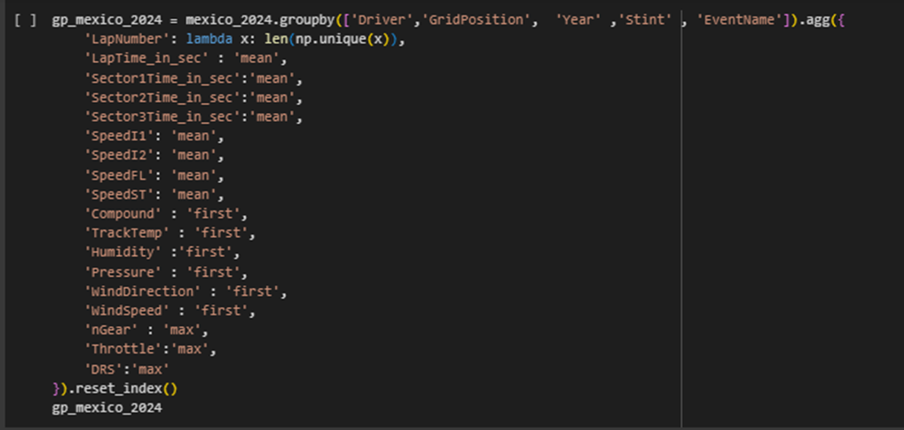
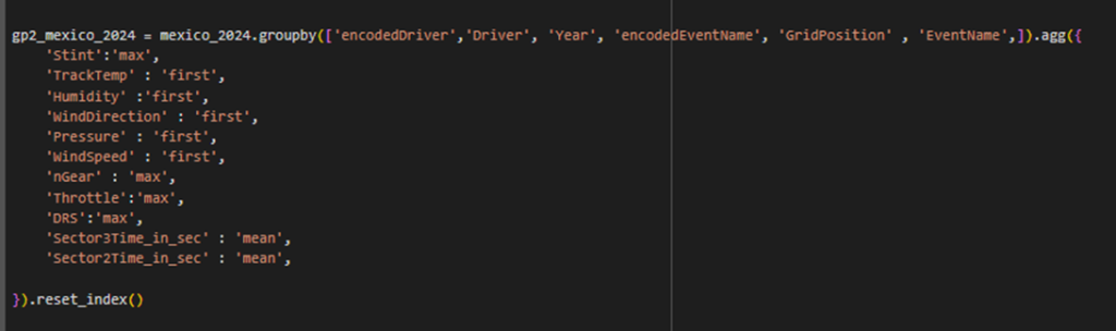
- we applied a groupby operation on the merged dataset to prepare the dataset for our model as follow which resulted a 1085 rows × 23 columns dataset.
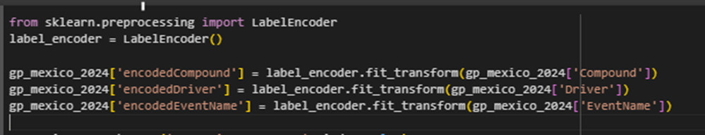
- after that, we performed a label encoding approach to categorical features like compound, events and drivers
- In the last, we removed all rows with at least one NaN value in it. There were 57 rows with NaN values and after dropping these rows a dataset with 1028 rows × 23 columns was achieved.
We used this final dataset as an input of our models to predict the targets
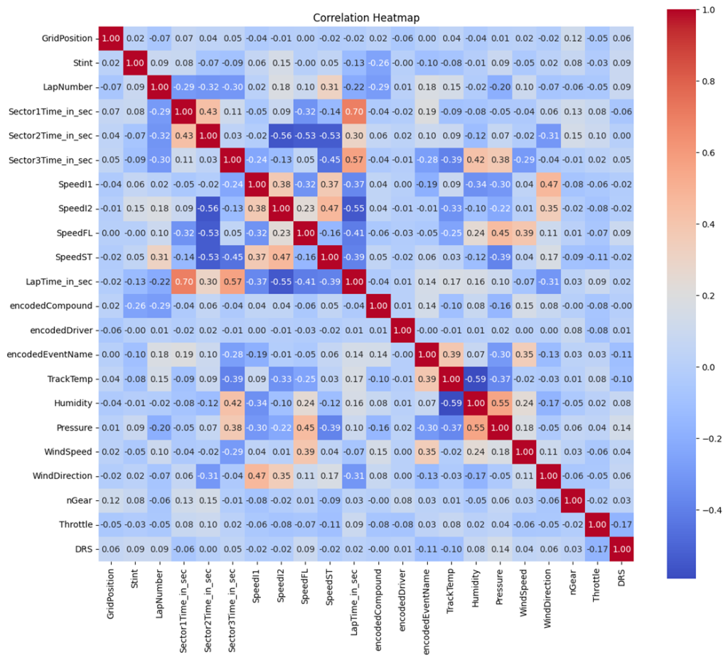
This is the correlation matrix of the final merged datasets, based on this :
- LapTime_in_sec
- Strongly correlated with Sector1Time_in_sec, Sector2Time_in_sec, and Sector3Time_in_sec (close to 0.7–0.9).
- This makes sense since lap time is the sum of these sector times.
- Sector Times
- All three sector times are highly correlated with each other (around 0.5–0.6).
- This suggests that consistent performance in one sector tends to reflect on others.
- Speed Relationships
- SpeedFL (Front Left) and SpeedST (Straight-line speed) show moderate correlations (0.3–0.5) with lap times and sector times.
- Higher straight-line speed tends to result in better lap times.
- Environmental Factors
- TrackTemp shows a mild correlation with LapTime_in_sec (-0.3). Warmer tracks might slightly improve lap times.
- Humidity, pressure, and wind speed have weaker correlations, meaning they might not significantly impact performance.
- Grid Position
- Very low correlations with most performance metrics. Starting position doesn’t strongly reflect lap times directly in this dataset.
- Tire Compounds
- Encoded compounds show small correlations with lap times, hinting that tire selection slightly affects performance but isn’t the sole driver.
- Throttle and DRS
- Throttle and DRS have weak correlations with lap times, suggesting these metrics may not dominate the dataset or reflect strategic use during a race.
Models
The goal of this challenge is to train models to predict four targets : Stint , Compound , Average LapTime per Stint and LapNumber.
Since the tire compound , Lap Time and Lap Number relies on Stint-Number we aimed to first predict the number of Stints for each driver in each event. To do so we extracted the most correlated and useful features with stints.
| Stint | |
| encodedCompound | -0.255054 |
| LapTime_in_sec | -0.133948 |
| encodedEventName | -0.102583 |
| Sector3Time_in_sec | -0.092505 |
| TrackTemp | -0.078806 |
| Sector2Time_in_sec | -0.071660 |
| WindSpeed | -0.049698 |
| Throttle | -0.028036 |
| Humidity | -0.013828 |
| SpeedFL | -0.000489 |
| encodedDriver | -0.000353 |
| WindDirection | 0.018218 |
| GridPosition | 0.022576 |
| SpeedST | 0.051877 |
| SpeedI1 | 0.063822 |
| nGear | 0.077958 |
| Sector1Time_in_sec | 0.084926 |
| Pressure | 0.085867 |
| LapNumber | 0.086923 |
| DRS | 0.090269 |
| Year | 0.098323 |
| SpeedI2 | 0.148956 |
| Stint | 1.000000 |
Here is a list of features with their correlation with stints. Among all accessible features before starting the race, there are a few features that are influential and might help in accurate predicting. That leaded us to first predict some features such as Speeds features and Sectors-Times and then with the help of these predicted features we hoped we could better estimate the Stint number.
Sector Times
To predict Sectors-Time and Speeds we extract their correlated features and started our modelling with the most independent one. Among three sector times features and four speed features Sector3Time is the most independent feature. So we start with this one:
Sector3Time
| Sector3Time_in_sec | |
| SpeedST | -0.454139 |
| TrackTemp | -0.390382 |
| LapNumber | -0.300896 |
| WindSpeed | -0.293430 |
| encodedEventName | -0.275344 |
| SpeedI1 | -0.237529 |
| SpeedI2 | -0.126747 |
| Stint | -0.092505 |
| WindDirection | -0.044660 |
| encodedCompound | -0.044083 |
| nGear | -0.014729 |
| encodedDriver | -0.008817 |
| Throttle | 0.021384 |
| Sector2Time_in_sec | 0.033624 |
| SpeedFL | 0.046761 |
| DRS | 0.046824 |
| GridPosition | 0.048225 |
| Sector1Time_in_sec | 0.110925 |
| Year | 0.303668 |
| Pressure | 0.376581 |
| Humidity | 0.417945 |
| LapTime_in_sec | 0.568297 |
| Sector3Time_in_sec | 1.000000 |
Track-Temp, wind-speed , event-Name, Humidity and pressure are features with moderate correlation with sector3Time (near 0.3) and, ‘GridPosition‘, ‘WindDirection‘ , ‘encodedDriver‘, ‘DRS’ are features with low correlation but were used in modelling since they improved the accuracy.
- We performed Random Forest regressor and XGboost regressor on these features with grid search and 5folds CV.
- We picked 2023 Mexico race as test-data and the rest of data as train-data.
- Mse results of both RFR and XGboost indicate that both models perform relatively good and we can use the predicted sector3Time as an input features of our models to predict other features.
- Mse with RFR : 3.0096
- Mse with XGB : 4.3752
Note that all sector times and Lap time are converted to seconds and we predict them in seconds (the original format was time-delta)
Sector2Time
| Sector2Time_in_sec | |
| SpeedI2 | -0.560005 |
| SpeedST | -0.534200 |
| SpeedFL | -0.532940 |
| LapNumber | -0.318775 |
| WindDirection | -0.306351 |
| Humidity | -0.120836 |
| Stint | -0.071660 |
| WindSpeed | -0.022068 |
| SpeedI1 | -0.019948 |
| DRS | 0.000811 |
| encodedDriver | 0.023058 |
| Sector3Time_in_sec | 0.033624 |
| GridPosition | 0.038007 |
| encodedCompound | 0.056461 |
| Pressure | 0.069676 |
| Year | 0.081893 |
| TrackTemp | 0.090428 |
| encodedEventName | 0.099616 |
| Throttle | 0.103309 |
| nGear | 0.145298 |
| LapTime_in_sec | 0.301521 |
| Sector1Time_in_sec | 0.432706 |
| Sector2Time_in_sec | 1.000000 |
Sector2Time is the next independent feature that we selected for prediction. With the set of [‘WindDirection‘ , ‘Humidity‘ , ‘WindSpeed‘, ‘nGear‘ , ‘Throttle‘ ,’encodedEventName‘ , ‘TrackTemp‘, ‘Pressure‘ , ‘DRS‘, ‘encodedDriver’] as the input features we achieved the following accuracy with RFR and XGboost.
- Mse with RFR : 7.6311
- Mse with XGB : 16.0516
We selected Sector2Time to be the input features of the models for predicting main targets
Sector1Time
| Sector1Time_in_sec | |
| SpeedFL | -0.322526 |
| LapNumber | -0.292171 |
| SpeedST | -0.142095 |
| TrackTemp | -0.091265 |
| Humidity | -0.078078 |
| Year | -0.070808 |
| DRS | -0.064391 |
| SpeedI1 | -0.054475 |
| Pressure | -0.045374 |
| WindSpeed | -0.041062 |
| encodedCompound | -0.037002 |
| encodedDriver | -0.016631 |
| WindDirection | 0.060672 |
| GridPosition | 0.065376 |
| Throttle | 0.082594 |
| Stint | 0.084926 |
| SpeedI2 | 0.090479 |
| Sector3Time_in_sec | 0.110925 |
| nGear | 0.125177 |
| encodedEventName | 0.194175 |
| Sector2Time_in_sec | 0.432706 |
| LapTime_in_sec | 0.697245 |
| Sector1Time_in_sec | 1.000000 |
Sector1Time also is a good feature that can be used in predicting other targets. Selected input features for predicting Sector2Time are : [‘TrackTemp‘, ‘encodedEventName‘ , ‘nGear‘ ,’Humidity‘ , ‘DRS‘ , ‘Sector3Time_in_sec‘ , ‘Pressure‘ , ‘Throttle‘, ‘GridPosition’]
Xgboost significantly outperforms Random Forest model in predicting Sector1Time therefore we selected Xgboost as our predictor of Sector1Time and picked the predicted outputs of Xgboost as the input features to predict other factors
- Mse with RFR : 103.2037
- Mse with XGB : 13.7545
Speed Features
Neither of RFR nor XGboost could be trained well on data to predict the four speed features (SpeedI1, SpeedI2, SpeedST, SpeedFL). With the examination of various combinations of input features and applying grid search on selecting the parameters, the mse score on these features didn’t goes well so we didn’t involve these feature as the inputs of our further models.
Stint
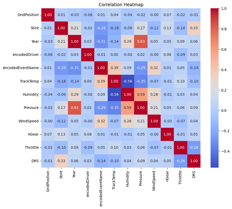
To predict Stint Number we change the final merged dataset in a way that we access the total number of Stint for each driver per event. In this regard we applied a group-by method one more time and obtained a new smaller dataset with 399 rows ×17 columns.
We then split the data into test and train where 2023 Mexico data was considered as test data. Test data contains 20 samples and train data 377 samples. Also we did 5fold CV to prevent overfitting and estimate the model performance better.
| Stint | |
| encodedCompound | -0.255054 |
| LapTime_in_sec | -0.133948 |
| encodedEventName | -0.102583 |
| Sector3Time_in_sec | -0.092505 |
| TrackTemp | -0.078806 |
| Sector2Time_in_sec | -0.071660 |
| WindSpeed | -0.049698 |
| Throttle | -0.028036 |
| Humidity | -0.013828 |
| SpeedFL | -0.000489 |
| encodedDriver | -0.000353 |
| WindDirection | 0.018218 |
| GridPosition | 0.022576 |
| SpeedST | 0.051877 |
| SpeedI1 | 0.063822 |
| nGear | 0.077958 |
| Sector1Time_in_sec | 0.084926 |
| Pressure | 0.085867 |
| LapNumber | 0.086923 |
| DRS | 0.090269 |
| Year | 0.098323 |
| SpeedI2 | 0.148956 |
| Stint | 1.000000 |
we used wrapper method for feature selection both in forward and backward approach and these features are the final selected features to do modelling: [‘encodedDriver‘, ‘GridPosition‘, ‘TrackTemp‘, ‘WindDirection‘, ‘nGear‘, ‘Throttle‘, ‘DRS‘, ‘Humidity‘, ‘Pressure‘, ‘WindSpeed’ ] which are described below :
- encodedDriver: this is the encoded feature of each driver name which is encoded by labelEncoder module of sklearn library.
- GridPosition : the starting position of each driver in the beggining of the race which are determined after qualifying race
- TrackTemp: indicates the temperature of track just in the start of the race (instead of calculating temperature mean value we calculate first value which is accessible before the race)
- WindDirection : this value also showd the direction of wind in the race track and like TrackTemp we consider its value in the beginning of the race by using ‘first’ at group-by method.
- nGear, Throttle, DRS, : these three values related with the car statistics and we used the maximum value of each in our modelling
- Humidity, Pressure, WindSpeed : the same as track temperature and wind direction , we considered their values in the start of the race since the predictor doesn’t know the mean of these values just in the beginning and he only accesses to their value just at the time.
Before training a model on input data to predict Stint Number, we did a grid search to find the best parameters for our models. We trained three different well-know classifiers on data to classify the number of stints (5 classes ) and selected the best two models outputs for predicting compounds , LapTimes and lapNumbers. We used accuracy score as our metric.
Here are the results and the parameters of each models :
- SVM Classifier:
- Best hyperparameters: {‘C’: 100, ‘gamma’: 0.1, ‘kernel’: ‘rbf’}
- Cross-validation accuracyscores: [0.55 0.7 0.7375 0.65 0.62025316]
- Accuracy on test data : 0.7000
- Xgboost Classifier :
- Best hyperparameters: {‘learning_rate’: 0.01, ‘max_depth’: 3, ‘min_child_weight’: 5, ‘n_estimators’: 500}
- Cross-validation scores: [0.6125 0.625 0.8 0.7 0.67088608]
- Accuracy on test data : 0.6000
- RandomForest Classifier:
- Best hyperparameters: {‘max_depth’: 5, ‘min_samples_leaf’: 1, ‘min_samples_split’: 10, ‘n_estimators’: 1000}
- Cross-validation scores: [0.625 0.4 0.3625 0.3875 0.41772152]
- Accuracy on test data : 0.1000
Compound
To predict tire compounds, we used the final merged dataset with 1028 × 23 rows . As before we picked 2023 Mexico data as test data with 54 samples and the remaining data as train data with 974 samples. We applied SVM, RF and XGBoost classifiers on our data and picked the predicted values of best classifier as the input feature for predicting average lapTime and LapNumber.
We used the predicted Stint values in our test data and since the predicted stints may be different from the actual stints, number of samples in test data would vary from the original test data based on the stint number. In this regard , we manipulated the test data as follows:
We added a new column to the dataset called ‘Stints.’ This column was populated based on the predicted stint values. If a driver has a predicted stint value of 3, there should be three corresponding rows for that driver. If the original dataset contained two rows, we added an additional row based on the existing data and populated the other features by fill-forward method. Conversely, if there were four rows in original data, we removed the last row to align with the predicted stint count. Finally, we filled the ‘Stints’ column for each driver in ascending order from 1 to the predicted stint number. For instance, for a driver with a predicted stint value of 3, there would be three rows with values 1, 2, and 3 in the ‘Stints’ column.
We did the same while predicting LapTime and LapNumber.
| encodedCompound | |
| LapNumber | -0.288121 |
| Stint | -0.255054 |
| Year | -0.251772 |
| Pressure | -0.155061 |
| TrackTemp | -0.104652 |
| Throttle | -0.075142 |
| SpeedFL | -0.057745 |
| Sector3Time_in_sec | -0.044083 |
| LapTime_in_sec | -0.037200 |
| Sector1Time_in_sec | -0.037002 |
| DRS | -0.002745 |
| nGear | -0.001490 |
| encodedDriver | 0.009635 |
| GridPosition | 0.019327 |
| SpeedI1 | 0.042534 |
| SpeedI2 | 0.043905 |
| SpeedST | 0.052232 |
| Sector2Time_in_sec | 0.056461 |
| WindDirection | 0.080196 |
| Humidity | 0.082962 |
| encodedEventName | 0.140700 |
| WindSpeed | 0.152087 |
| encodedCompound | 1.000000 |
Here are a list of input features to predict compounds:
[encodedDriver, encodedEventName, GridPosition, TrackTemp, Humidity, WindDirection, Pressure, WindSpeed, nGear, Throttle, DRS, Sector3Time_in_sec, Sector2Time_in_sec, Sector1Time_in_sec, Stint]
Note that:
- Sector3Time_in_sec, Sector2Time_in_sec, Sector1Time_in_sec and Stint are predicted values which are replaced with the original features in test data.
- we train the model with actual values of Sector3Time_in_sec, Sector2Time_in_sec, Sector1Time_in_sec and Stint but while we want to predict the test data, we replace the previous predicted values in test data.
- Since the 3 predicted sector-times features have equal length with test data we first replaced them with actual sector-times and then we manipulate the test for replacing the predicted stint values in a way that we described before .
Here are the results and the parameters of each models :
- Xgboost Classifier :
- Best hyperparameters: {max_depth= 10, min_samples_leaf= 1, min_samples_split= 2, n_estimators= 500}
- Cross-validation accuracy scores: [0.63592233 0.76699029 0.75242718 0.78536585 0.67317073]
- Accuracy on test data : 0.7627
- RandomForest Classifier:
- Best hyperparameters: { max_depth=5, min_samples_leaf=2, min_samples_split=2, n_estimators=100, random_state=42}
- Cross-validation accuracy scores: [0.69417476 0.70873786 0.71359223 0.72195122 0.70731707]
- Accuracy on test data : 0.8235
- SVM Classifier: (we didn’t use this model since cv score are significantly lower than test score)
- Best hyperparameters: C= 1, kernel=’rbf’, gamma= 0.1
- Cross-validation scores: [0.36893204 0.37378641 0.4368932 0.37560976 0.35609756]
- accuracy_score on test set: 0.8235
Average Lap Time
To predict tire LapTime, we used the original merged dataset with 1028 × 23 rows. As before we picked 2023 Mexico data as test data with 54 samples and the remaining data as train data with 974 samples. We applied SVM, RF and XGBoost regressors on our data and picked the predicted values of best regressor as the input feature for predicting LapNumber.
- We used the predicted Stint number, and predicted sector times in our test data in the way that we discussed before.
- After manipulating the test data by inserting the predicted stint number for each driver we added the predicted encoded compounds to it (replace with real one in test data)
- All sector times and Lap time are converted to seconds and we predict them in seconds not in delta time
| LapTime_in_sec | |
| SpeedI2 | -0.545752 |
| SpeedFL | -0.408371 |
| SpeedST | -0.389099 |
| SpeedI1 | -0.368425 |
| WindDirection | -0.309157 |
| LapNumber | -0.218260 |
| Stint | -0.133948 |
| WindSpeed | -0.072634 |
| encodedCompound | -0.037200 |
| GridPosition | -0.018013 |
| encodedDriver | 0.008118 |
| DRS | 0.018156 |
| nGear | 0.026198 |
| Year | 0.063681 |
| Throttle | 0.094519 |
| Pressure | 0.100717 |
| encodedEventName | 0.141955 |
| Humidity | 0.159217 |
| TrackTemp | 0.167180 |
| Sector2Time_in_sec | 0.301521 |
| Sector3Time_in_sec | 0.568297 |
| Sector1Time_in_sec | 0.697245 |
| LapTime_in_sec | 1.000000 |
These are the input features that we have used for our three regressor models:
[‘encodedDriver‘ , ‘encodedEventName’, ‘GridPosition’ ,’TrackTemp’, ‘Humidity‘ ,’WindDirection’, ‘Pressure’ ,’WindSpeed’,’nGear’, ‘Throttle’ ,’DRS’, ‘Sector3Time_in_sec’, ‘Sector2Time_in_sec’, ‘Sector1Time_in_sec’, ‘Stint‘, ‘encodedCompound‘]
And here are the results and the parameters of each models :
- Xgboost Regressor :
- Best hyperparameters: {‘learning_rate’: 0.1, ‘max_depth’: 3, ‘min_child_weight’: 1, ‘n_estimators’: 200}
- Cross-validation MSE scores: [3.02127283 2.53466101 1.24585892 0.93771299 3.75053471]
- MSE score on test set: 2.4089
- RandomForest Regressor :
- Best hyperparameters: {‘max_depth’: 15, ‘min_samples_leaf’: 1, ‘min_samples_split’: 2, ‘n_estimators’: 200}
- Cross-validation MSE scores: [2.93043564 2.34767154 1.45211941 1.22731235 4.75973872]
- MSE score on test set: 4.6621
- SVM Regressor :
- Best hyperparameters: {‘C’: 0.1, ‘epsilon’: 0.5, ‘gamma’: 0.001, ‘kernel’: ‘linear’}
- Cross-validation scores: [0.48926279 5.37217463 0.95356296 1.43544879 0.64799476]
- mean_squared_error on test set: 3.0170
Lap Number
To predict tire LapNumber, we used the original merged dataset with 1028 × 23 rows. As before we picked 2023 Mexico data as test data with 54 samples and the remaining data as train data with 974 samples. We applied SVM, RF and XGBoost regressors on our data.
- we used the predicted Stint number, and predicted sector times in our test data in the way that we discussed before.
- After manipulating the test data by stint number we added predicted encoded compounds and predicted Average Lap-Time to it (replace with real one in test data)
| LapNumber | |
| Sector2Time_in_sec | -0.318775 |
| Sector3Time_in_sec | -0.300896 |
| Sector1Time_in_sec | -0.292171 |
| encodedCompound | -0.288121 |
| LapTime_in_sec | -0.218260 |
| Pressure | -0.199534 |
| Year | -0.190465 |
| WindDirection | -0.071647 |
| GridPosition | -0.069630 |
| nGear | -0.058414 |
| Throttle | -0.053525 |
| Humidity | -0.022797 |
| encodedDriver | 0.010552 |
| SpeedI1 | 0.018405 |
| Stint | 0.086923 |
| DRS | 0.087992 |
| WindSpeed | 0.099560 |
| SpeedFL | 0.099857 |
| TrackTemp | 0.146897 |
| encodedEventName | 0.177722 |
| SpeedI2 | 0.179566 |
| SpeedST | 0.314533 |
| LapNumber | 1.000000 |
These are the input features that we have used for our three regressor models:
[‘encodedDriver‘, ‘encodedEventName’, ‘GridPosition’, ‘TrackTemp’, ‘Humidity’ , ‘WindDirection’, ‘Pressure‘ ,’WindSpeed’ ,’nGear’, ‘Throttle’ ,’DRS’, ‘Stint‘, ‘encodedCompound‘, ‘LapTime_in_sec‘ ]
We trained three different well-know regressors on data to predict the Lap Number. We used MSE score as our metric.
Here are the results and the parameters of each models :
- Xgboost Regressor :
- Best hyperparameters: {‘learning_rate’: 0.1, ‘max_depth’: 5, ‘min_child_weight’: 5, ‘n_estimators’: 100}
- Cross-validation MSE scores: [62.35517616 56.07027669 39.75775935 47.1023616 74.11965767]
- MSE score on test set: 107.3121
- RandomForest Regressor :
- Best hyperparameters: {‘max_depth’: 15, ‘min_samples_leaf’: 2, ‘min_samples_split’: 5, ‘n_estimators’: 100, random_state=42}
- Cross-validation MSE scores: [61.41047762 60.89041624 41.07036987 43.82738211 85.71943427]
- MSE score on test set: 80.3144
- SVM Regressor : (worst CV scores , best test score 😀 )
- Best hyperparameters: {‘C’: 100, ‘epsilon’: 0.5, ‘gamma’: 0.1, ‘kernel’: rbf’}
- Cross-validation scores: [171.34258869 147.24932474 127.19217298 156.75709082 148.07181069]
- mean_squared_error on test set: 48.5515
Conclusion and Final Tips
In this article, we tried to explore the exciting world of the 2024 Mexico City Formula 1 race prediction using AI and Ocean Protocol. The insights provided are intriguing, but there’s always room for improvement, such as enhancing data accuracy and incorporating more diverse datasets for better predictions.
Future work could focus on refining the algorithms and expanding the analysis to include more variables, which would provide an even clearer picture of race outcomes. Overall, this journey into AI and racing is just the beginning, and we look forward to seeing how technology evolves in this thrilling sport!